International Journal of Scientific & Engineering Research Volume 2, Issue 7, July-2011 1

ISSN 2229-5518

Weather Forecasting using ANN and PSO

Asis Kumar Tripathy, Suvendu Mohapatra, Shradhananda Beura, Gunanidhi Pradhan

Abstract— Weather prediction is basically based upon the historical time series data. The basic parameters of weather prediction are max- imum temperature, minimum temperature, rainfall, humidity etc. In this paper we are trying to predict the future weather condition based upon above parameters by Artificial Neural Network and Particle Swarm Optimization Technique. The basic Data mining operations are employed to get a useful pattern from a huge volume of data set. Different testing and training scenarios are performed to obtain the accurate result. Experimental results indicate that the proposed approach is useful for weather forecasting.

Index Terms— Weather forecasting, Artificial Neural Network, Particle Swarm Optimization Technique, Data mining, Numerical

Weather Prediction, Network Forecasting

1 INTRODUCTION

—————————— • ——————————
eather forecasting is the application of science and technology to predict the state of the atmosphere for a future time and a given location. Human be-
ings have attempted to predict the weather informally for millennia, and formally since at least the nineteenth cen- tury. Weather forecasts are made by collecting quantita- tive data about the current state of the atmosphere and using scientific understanding of atmospheric processes to predict how the atmosphere will evolve. Weather fore- casting is an ever-challenging area of investigation for scientists. In this research a weather forecasting model using Neural Network is going to propose. The weather parameters like maximum temperature, minimum tem- perature, relative humidity and rainfall is going to pre- dicted using the features extracted over different periods as well as from the weather parameter time-series itself. The approach applied here uses feed forward artificial neural networks (ANNs) with back propagation for su- pervised learning using the data recorded at a particular station. The trained ANN was used to predict the future weather conditions. The model can be suitably adapted for making forecasts over larger geographical areas. Weather changes affect also the demand for electricity. Typically, weather variables are used in the prediction of demand for electricity. The predictions are based on neural network and statistical modeling. The results indi- cate that, in some cases, the effect of weather is indirectly

————————————————

• Asis Kumar Tripathy is currently working as a Lecturer in dept of IT in

NMIET Bhubaneswar, India, E-mail: asistripathy@gmail.com

• Suvendu Mohapatra is currently working as a software developer in Mind- fire solutions, Bhubaneswar,India,E-mail: mohapatra.suvendu@gmail.com

• Shradhananda Beura is currently working as a lecturer in IT in NMIET Bhubaneswar,India,E-mail:beura.shradhananda@gmail.com

• Gunanindhi Pradhan is currently working as Principal Govt. College of

Engineering Kalahandi, India, E-mail: gunanidhi_p@rediffmail.com
taken into account by other variables, and explicit use of weather variables may not be necessary. However, the decision to include or exclude weather variables should be analyzed for each individual situation.

1.1 Weather Forecasting System

1.1.1 Weather Data collection

Observations of atmospheric pressure, temperature, wind speed, wind direction, humidity, and precipitation are made near the earth's surface by trained observers, auto- matic weather stations. The World Meteorological Organ- ization acts to standardize the instrumentation, observing practices and timing of these observations worldwide.

1.1.2 Weather Data Assimilation

During the data assimilation process, information gained from the observations is used in conjunction with a nu- merical model's most recent forecast for the time that ob- servations were made to produce the meteorological analysis. This is the best estimate of the current state of the atmosphere. It is a three dimensional representation of the distribution of temperature, moisture and wind.

1.1.3 Numerical Weather Prediction

Numerical Weather Prediction (NWP) uses the power of computers to make a forecast. Complex computer pro- grams, also known as forecast models, run on supercom- puters and provide predictions on many atmospheric variables such as temperature, pressure, wind, and rain- fall. A forecaster examines how the features predicted by the computer will interact to produce the day's weather.

2 LITERATURE REVIEW

Back Propagation was introduced by Rumelhart and Hin- ton in 1986. It is the most widely used network today. The basic idea in back propagation network is that the neu- rons of lower layer send up their outputs to the next layer. It is a fully connected, feed forward, hierarchical

International Journal of Scientific & Engineering Research Volume 2, Issue 7, July-2011 2

ISSN 2229-5518

multi layer network, with hidden layers and no intra- connections.
. PSO was developed by Dr. Russell Eberhart and Dr. James Kennedy in 1995. PSO is based upon the popula- tion for numerical optimization without explicit know- ledge of the problem. This stochastic optimization tech- nique was inspired by the social behavior and intelligence of swarms.
Kennedy and Eberhart (1997) described a very simple
alteration of the canonical algorithm that operates on bit- strings rather than real numbers. In their version, the ve- locity is used as a probability threshold to determine whether xid the dth component of xi should be evaluated as a zero or a one.
Kennedy and Spears (1998) compared this binary particle swarm to several kinds of GAs, using Spears’ multimodal random problem generator. This paradigm allows the creation of random binary problems with some specified characteristics, e.g., number of local optima, dimension, etc.
Mohan and Al-Kazemi (2001) suggested several ways that
the particle swarm could be implemented on binary spac-
es. One version, which he calls the “regulated discrete
particle swarm,” performed very well on a suite of test
problems.
Agrafiotis and Cedeño (2002) used the locations of the
particles as probabilities to select features in a pattern-
matching task. Each feature was assigned a slice of a rou-
lette wheel based on its floating-point value, which was
then discretized to {0, 1}, indicating whether the feature
was selected or not.
In Pamparä et al. (2005), instead of directly encoding bit
strings in the particles, each particle stored the small
number of coefficients of a trigonometric model (angle
modulation) which was then run to generate bit strings.
Extending PSO to more complex combinatorial search spaces is also of great interest.
Parrot and Li (2006) adjust the size and number of swarms dynamically by ordering the particles into ‘spe- cies’ in a technique called clearing. Blackwell and Branke
(2006), borrowing from the atomic analogy referred to above, invoke an exclusion principle to prevent swarms from competing on the same peak and an anti- convergence measure to maintain diversity of the multi- swarm as a whole.
Recently, a self-adapting multi-swarm has been derived
(Blackwell 2007)[3]. The multi-swarm with exclusion has been favorably compared, on the moving peaks problem, to the hierarchical swarm, PSO re-initialization and a state of the-art dynamic-optimization evolutionary algorithm known as self-organizing scouts.

3 ARTIFICIAL NEURAL NETWORK

3.1 Definition

A neural network is a system composed of many simple processing elements operating in parallel whose function is determined by network structure, connection strength and the processing performed at computing elements or nodes.
A neural network is a massively parallel distributed
processor made up of simple processing units, which has
a neutral property fro storing experiential knowledge and
making it available for use. It resembles the brain in two
aspects-
1. Knowledge is acquired by the network from its
environment through a learning process.
2. Interneurons connection strengths, known as
synaptic weights ,are used to store the acquired
knowledge.

3.2 Characteristics Neural networks

3. Neural network is composed of large number of very simple processing elements called neurons
4. Each neuron is connected to other neuron by means of interconnections or links with an asso- ciated weights.
5. Memories are stored or represented in a neural
network in the pattern of interconnections or
links with an associated weight.
6. Interconnections are processed by changing the
strength of interconnection and/or changing the state of each neuron.
7. A neural network is trained rather than pro- grammed.
8. A neural network act as associative memory i.e it

stores information by associating it with other in- formation in the memory.
BIOLOGICAL

International Journal of Scientific & Engineering Research Volume 2, Issue 7, July-2011 3

ISSN 2229-5518

ARTIFICIAL
Figure 3.1: Analogy of Biological and Artificial Neuron
9. It is robust as its performance doesn’t degrade appreciably if some of its neurons or interconnec- tion are lost(distributed memory).
10. Neural network are capable to recall information based on incomplete or noisy or partially incor- rect inputs.
11. A neural network can be self organizing i.e. some neural networks can be made to generalize from data patterns used in training without being pro- vided with specific instructions on exactly what to learn.

4 PARTICLE SWARM OPTIMIZATION (PSO)

4.1 Introduction

Particle Swarm Optimization (PSO) was only a few years ago a curiosity, has now attracted the interest of research- ers around the globe. PSO was developed by Dr. Russell Eberhart and Dr. James Kennedy in 1995. PSO is based upon the population for numerical optimization without explicit knowledge of the problem. This stochastic opti- mization technique was inspired by the social behavior and intelligence of swarms. This simple concept is a effi- cient method for solving many different optimization problem.
PSO gives the solution towards much similar kind of
problems such as Genetic Algorithms. It needs only ma-
thematical operations and computationally inexpensive with respect to memory and speed. Initially the system holds random solutions and gradually update it’s genera- tions to find the optimal solutions.

4.2 PSO Workflow

In PSO a number of simple entities the particles are placed in the search space of some problem or function, and each evaluates the objective function at its current location. Each particle then determines its movement through the search space by combining some aspect of the history of its own current and best (best-fitness) locations with those of one or more members of the swarm, with some random perturbations. The next iteration takes
place after all particles have been moved. Eventually the swarm as a whole, like a flock of birds collectively forag- ing for food, is likely to move close to an optimum of the fitness function.
Each individual in the particle swarm is composed of
three D-dimensional vectors, where D is the dimensional-
ity of the search space. These are the current position xi,
the previous best position pi, and the velocity vi. The cur-
rent position xi can be considered as a set of coordinates
describing a point in space. On each iteration of the algo- rithm, the current position is evaluated as a problem solu- tion. If that position is better than any that has been found so far, then the coordinates are stored in the second vec- tor, pi. The value of the best function result so far is stored in a variable that can be called pbesti (for “pre- vious best”), for comparison on later iterations.

5 WEATHER FORECASTING USING ANN AND PSO

5.1 Definition

Weather plays a vital role for agriculture sector and many other industries. India is an agro economy based country. So weather prediction should be more accurate. Weather is the state of atmosphere of a particular place and time. Weather parameters are collected from the various sta- tions of meteorological department, Orissa. The basic pa- rameters are maximum temperature, minimum tempera- ture, rainfall, humidity, pressure and cloudiness. There many forecasting models are present which uses Artificial Neural Network (ANNs). In this project a model is pro- posed which uses ANNs and Particle Swarm Optimiza- tion (PSO) technique for better results. This prediction is only for particular stations of Orissa state.
Traditional techniques of prediction are failed for non linear data sets. ANN gives the flexibility to solve that
kind of problems. It is very difficult for the traditional technique to identify the condition between input and output parameters but ANN has the capability to extract the relation between input and output.
ANN uses biological neurons for intensive computation. Neural network adjust their weights by process of train-
ing. I am using PSO for better optimization of weights. We are more interested to reduce the total error with little tolerance. The network is trained in such a manner that the model should give the optimum results. After training the model is used for testing which produces appropriate results.

5.2 Neural Network Designing for Weather

Forecasting using PSO

In this section an implantation for weather forecasting is introduced using three different neural network architec- tures, namely, RBF and backpropagation neural net- works. For this purpose different case studies are imple- mented for both neural networks architectures.

International Journal of Scientific & Engineering Research Volume 2, Issue 7, July-2011 4

ISSN 2229-5518

5.2.1 Neural Network

The proposed model uses Multilayer Feed forward archi- tecture that has one hidden layer (layers between input layer and output layer), whose computation nodes are hidden neurons also termed as hidden units. The features extracted from weather data are applied as input samples and the target is taken as the parameter to be estimated during training operation. Particle Swarm Intelligent is a population based heuristic optimization technique in which each particle represents a solution within a search space. This technique was used to optimize the weights in the neural network so that we got the better results.
The simulation procedure using back propagation net-
work is divided into two steps, the first one first consider
the selection of network setting parameters. The second one considers the using of this network in forecasting at different training and testing scenarios. The details of those two steps are given in the following subsections.

5.2.1.2 Network Parameters Setting

In this simulation, the implemented back propagation network has a single hidden layer with 10 nodes. Each node in the hidden layer use Gaussian function as basis functions. The basis centers are selected from the input data which are used to train the network. The weighting vectors are initialized with random values. The learning of the network is based on the back propagation algo- rithm.
The back propagation network is built using Matlab and defining our own code for neural network design, so the
following architecture parameters must be specified.
12. Number of inputs: this parameter sets the num-
ber of units allocated for the input layer. It must
be an integer value greater than or equal to 1.
13. Number of basis units in the hidden layer: this
parameter sets the number of basis units allo- cated for the hidden layer. It must be an integer value greater than or equal to zero.
14. Number of outputs: this parameter sets the num- ber of units allocated for the output layer. It must be an integer value greater than or equal to 1.

5.2.1.2 Network Forecasting

Daily data sets of 2008 (i.e. maximum, minimum tempera- ture and rainfall) of Orissa state were used as training set, and first two months of 2009 were used as test set of our neural network.
We use the minimum temperature, maximum tempera- ture and rainfall of different region of Orissa using only one year as at a training set namely 2008, in addition to the next day of the day we want to predict. Then we use the obtained network architecture and weights to test the ability of this network to predict the minimum tempera- ture, maximum temperature and rainfall for the next year (2009).

5.2.1.3 Model Implementation

The model is developed in MATLAB 7, and the code is done in Windows PC running on Windows XP. The mod- el takes input from the datasets and produces the result for both optimal weights and biases.
The model follows a standard feed forward network algo-
rithm together with PSO as optimization step for optimiz-
ing error. The algorithm is given below.
1. Iinitialize number of hidden neurons, popu- lation size, maximum iterations and model parameters(c1, c2,m)
2. Read weather and yield data from file
3. generate random population and biases
4. for each population i = 1, . . . , populationsize do
5. calculate fitness;
6. end for
7. calculate Population best(pbest) and Global
Best(gbest)
8. for i = 1, . . . , maxIterations do
9. for i = 1, . . . , populationsize do
10. for j = 1, . . . , dimensions do
11. Calculate velocity;
12. Calculate Position;
13. end for
14. end for
15. Calculate fitness value
16. for i = 1, . . . , populationsize do
17. Calculate population best(pbest)
18. end for
19. Calculate global best (gbest)
20. end for
21. Display final Weights and Biases

Fitness Function

The fitness function used for the model is a feed forward network. The feed forward network takes the number of input (generated weights and biases) and hidden neu- rons, weather data and calculates the error of the calcula- tion. The error is optimized by the PSO algorithm to find the final output.
feval = fitness_eval (w , input_data , d,no_of_input_neurons , no_of_hidden_neurons)
where , w = initial randomly generated weight popula- tion,
input_data = weather data from the dataset d = Total dimension of the population.
The Fitness_eval routione takes these parameters and calculates the error depending on the actual weather data. It returns the square error as its output. The squared error is passed as input to PSO for optimization.

5.3 Model Training

The training dataset formed out of 3 years of data is used for training the model. The various combination of net- work parameters are taken and is shown in Table.

International Journal of Scientific & Engineering Research Volume 2, Issue 7, July-2011 5

ISSN 2229-5518

Table 5.3: Various combination of network parameter

6 RESULTS OF RAINFALL

Fig 6.1 shows the training target and output from neural network model for estimating rainfall of Puri Zone for the year 2008. Both the curves overlap for most of data values which shows that output and target are very similar in values. During training all outputs are in error range less than 4%.
Fig 6.2 shows the testing target and output generated.
During testing 94% of estimated data points are closed to
desired data values.
These ANN models have the potential to be useful as a component of weather prediction like humidity, long range rainfall and temperature prediction, so it needs further development and validation.ANN modeling with additional locations will increase the variability and pos- sibly increase, the predictive capabilities of ANN-based weather prediction.

REFERENCES:

[1]. Paras, Sanjay Mathur, Avinash Kumar, and Mahesh Chandra. “A Feature Based Neural Network Model for Weather Forecasting”(2009). [2]. H. M. Abdul Kader. “Neural Networks Training Based on Diffe- rential Evolution Algorithms Compared with Other Architectures for Weather Forecasting34”. International Journal of Computer Science and

Network Security, VOL.9 No.3 March 2009.

[3]. Riccardo Poli · James Kennedy · Tim Blackwell, “Particle swarm optimization An overview” Received: 19 December 2006 / Accepted:

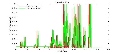
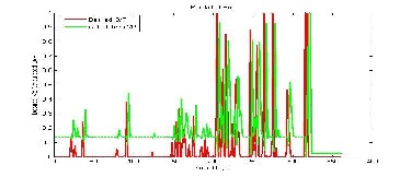
Figure 6.1: Rainfall of puri
Figure 6.2: Rainfall of Puri

7 CONCLUSION

ANN with PSO model produced consistently lower error rates with variation of 4 ± 1 % for yearly dataset. The overall error rate for the model is 4 % which is in the al- lowable error range. Testing of the prepared model gives an error rate of 5± 1 % on an overall basis. Improved ANN models were produced with training tolerances set high and gradually lowered as the networks trained.