International Journal of Scientific & Engineering Research, Volume 2, Issue 2, February-2011 1

ISSN 2229-5518

UTILITY OF PSO FOR LOSS MINIMIZATION AND ENHANCEMENT OF VOLTAGE PROFILE USING UPFC

A.S Kannan, R. Kayalvizhi

Abstract - The loss minimization is a major role in Power System (PS) research. Transmission line losses in a PS can be reduced by Var compensation. After the establishment of power markets with transmission open access, the significance and use of Flexible AC Transmission Systems (FACTS) devices for manipulating line power flows to relieve congestion and maximize the overall grid operation have been increased. This paper presents a method to provide simultaneous or individual controls of basic system parameters like transmission voltage, impedance and phase angle, which are controlling by using Unified Power Flow Controller (UPFC). The Particle Swarm Optimization (PSO) method is used to compute the power flow in optimum value. The performance of this technique is tested using IEEE - 14 bus system through the MatLab/Simulink simulation software package. The simulation results of test power system show that the location of the UPFC has been able to enhance the voltage level of the test power system and also minimize the transmission line losses.

Keywords - Flexible AC Transmission Systems (FACTS), Particle Swarm Optimization (PSO), Real and Reactive Power, Unified Power

Flow Controller (UPFC).

—————————— • ——————————

1. INTRODUCTION

Most of the large power system blackouts, which occurred worldwide over the last twenty years, which are caused by heavily stressed system with large amount of real and reactive power demand and low voltage condition. When the voltages at power system buses are low, the losses will also to be increased. This study is devoted to develop a technique for improving the voltage and minimizing the losses and hence eliminate voltage instability in a power system [4]. State estimation is the process of estimating the values to an unknown system variable based on the measurement system according to some criterion. The basic idea was to "fine-tune" state variables by minimizing the sum of the residual squares. This is the well-known least squares (LS) method; State estimation is a widely used tool in power system energy management systems. The essence of state estimation is that the measurements are taken of active and reactive power, and system voltage magnitudes and phase angles (i.e, the ‘states’) are estimated [1]-[2]. Application of FACTS devices are currently pursued very intensively to achieve better control over the transmission lines for manipulating power flows.

State estimation in power system can be formulated as a nonlinear weighted least squared errors (WLSE) problem representing the zero injections of buses and the zero active power exchange between the power system and FACTS devices. There are several kinds of FACTS devices. Thyristor-Controlled Series Capacitors (TCSC), Thyristor Controlled Phase Shifting Transformer (TCPST) and Static Var Compensator (SVC) can exert a voltage in series with the line and, therefore, can control the active power through a transmission line[3][15]. On the other hand UPFC has a series voltage source and a shunt voltage source, allowing independent control of the voltage magnitude, and the real and reactive power flows along a given transmission line. The UPFC was proposed for real-time control and dynamic compensation of ac transmission systems, providing the necessary functional flexibility required to solve many of the problems facing the utility industry. The UPFC consists of two switching converters, which in the implementations considered are voltage sourced inverters using Gate Turn-Off (GTO) thyristor switch [5]. Particle swarm optimization (PSO) is a population based stochastic optimization technique inspired by social behavior of bird
flocking or fish schooling. PSO is related to evolution-inspired problem solving techniques such as genetic algorithms [9].
In this paper Particle Swarm Optimization (PSO) technique is
introduced to optimize the measurement error vector. The proposed technique was tested on the IEEE 14 bus system and UPFC can be installed at any of the weakest voltage at load buses. For practical and economic considerations, the number of UPFC units is limited to one. Here UPFC is connected in between 9 in IEEE 14 bus system to perform the test.

2. BASIC CIRCUIT OF UPFC

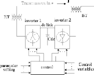
Fig. 1.Power Circuit of the Unified Power Flow Controller.
Fig.1 shows the power circuit of a UPFC which is composed of an Excitation Transformer (ET), a Boosting transformer (BT), two three phase GTO based voltage source converters (VSCs), and a dc link capacitor. This arrangement functions as an ideal ac to ac power converter in which the real power can freely flow in either direction between the ac terminals of the two inverters and each inverter can independently generate (or absorb) reactive power at its own ac output terminal . Inverter 1 can also generate or absorb controllable reactive power, if it is desired, and thereby it can provide independent shunt reactive compensation for the line. Inverter 2 provides the main function of the UPFC by injecting an ac voltage Vw with controllable magnitude Vm and phase angler (er)r at the power frequency, in search with line via an insertion transformer. This injected voltage can be considered essentially as a synchronous

IJSER © 2011 http://www.ijser.org

International Journal of Scientific & Engineering Research, Volume 2, Issue 2, February-2011 2

ISSN 2229-5518

ac voltage source [6]. The transmission line current flows through this voltage source resulting in real and reactive power exchange between it and the ac system. The real power exchanged at the ac
Sis = Vi (e-j(y+90)bserVi ) (7) Sis = V 2b r [cos(-y-90)+ j sin(-y-90)]. (8)

i se

By using trigonometric identities, Equation (8) reduces to:
terminal (i.e., at the terminal of the insertion transformer) is
Sis = -rbseVi

se i

converted by the inverter into dc power which appears at the dc link
as positive or negative real power demand. The reactive power exchanged at the ac terminal is generated internally by the inverter [7].

3. STEADY STATE MODEL OF UPFC

A UPFC can be represented in the steady-state by two voltage sources representing fundamental components of output voltage waveforms of the two converters and impedances being leakage reactances of the two coupling transformers. Figure 2 depicts a two voltage-source model of UPFC [5].

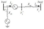
Figure 2. Two voltage-source model of UPFC
Voltage of bus i is taken as reference vector, Vi = Vi <0’ and Vi’ = Vse + Vi. The voltage sources, Vse and Vsh, are controllable in both their magnitudes and phase angles. The values of r and y are defined within specified limits given by Equation (1).
0 s: r s: rmax and 0 s: y s: 2n. (1) Vse should be defined as:

2 sin y - jrb V 2 cos y (9)

Equation (9) can be decomposed into its real and imaginary components,
Sis = Pis + jQis, where
Pis = -rbseVi sin y (10) Qis =-rbseV 2 cos y (11) Similar modifications can be applied to Equation (5); the final equation takes the form:
Sjs = ViVjbse r sin(8i - 8j + y) + jViVjbse r cos(8i - 8j + y) (12) Equation (12) can also be decomposed into its real and imaginary parts,
Sjs = Pjs + jQjs, where
Pjs = ViVjbser sin(8i - 8j + y) (13)
Qjs = ViVjbse r cos(8i - 8j + y) (14)

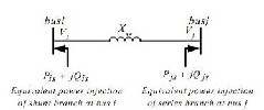
Figure 4. Equivalent power injections of series branch
In UPFC, the shunt branch is used mainly to provide both the real power, Pseries, which is injected to the system through the series branch, and the total losses within the UPFC. The total switching losses of the two converters is estimated to be about 2% of the power transferred, for thyristor based PWM convertors [12]. If the losses are to be included in the real power injection of the shunt connected voltage source at bus i, Pshunt is equal to 1.02 times the injected series
Vse = rViejy (2)
real power P

series

through the series connected voltage source to the
The steady-state UPFC mathematical model is developed by replacing voltage source Vse by a current source Ise parallel with the
system [9 - 10].
Pshunt =-1.02Pse ries (15)
The apparent power supplied by the series converter is calculated as
transmission line, where bse = 1/Xse.

Sseries = VseI * = rejyVi
(16)
Ise = -jbse Vse (3)
The current source Ise can be modeled by injection powers at the two auxiliary buses i and j as shown in Figure 3.
Active and reactive power supplied by the series converter can be calculated from Equation (16):
Sseries = rejyVi ((rejyVi - Vj) jXse)* (17)
Sseries = rViej (8i+y) ((rVie-j(8i+y)+Vie-j 8i - Vje-j 8j)l-jXse) (18)

2 + jb rV 2ejy - jb V V ej(8i-8j + y) (19)

Sseries = jbser2Vi

se i

se i j

Sis = Vi (-Ise)* (4) Sjs = Vj (-Ise)* (5)
Figure 3. Replacement of series voltage source by a current source
The injected powers Sis and Sjs can be simplified according to the following operations, by substituting Equation (2) and (3) into Equation (4).
Sis = Vi (jbse rViejy)* (6)
By using the Euler Identity, (ejy = cos y + J SIN y), Equation (6) takes the form:
The steady state model of UPFC consists of two ideal voltage sources, one in series and one in parallel with the associated line. Neglecting UPFC losses, during steady-state operation it neither absorbs nor injects real power into the system. No real-power is exchanged between the UPFC and the system. The two sources are mutually dependent. The real and reactive power going through line can be formulated by the equation (3).

4. PARTICLE SWARM OPTIMIZATION TECHNIQUE

PSO is basically developed through simulation of bird flocking in two dimension space. The position of each agent is represented by XY-axis position and the velocity is expressed by vx (the velocity of

IJSER © 2011 http://www.ijser.org

International Journal of Scientific & Engineering Research, Volume 2, Issue 2, February-2011 3

ISSN 2229-5518

2 2

X-axis) and vy (the velocity of Y-axis). Modification of the agent
position is realized by the position and velocity information. PSO
procedures based on the above concept can be described as follows. Namely, bird flocking optimizes a certain objective function. Each agent knows its best value so far (pbest) and its XY position.
PL-k=Gk(Vi +Vj -2ViVjcos(Oi-Oj)) (23)
The series reactive power loss equation of the kth line, between buses i and j can be written as,

2 2

Moreover, each agent knows the best value in the group (gbe st) among
pbests. Each agent tries to modify its position using the current velocity and the distance from pbest and gbest. The modification can be
represented by the concept of velocity. Velocity of each agent can be
modified by the following equation.[9]-[10] Vi=Vi + rand x (pbest
i – Si) + rand x (gbest – Si)
where, Vi : velocity of agent i,
rand : uniformly distributed random number between 0 and 1,
Si : current position of agent i, pbest i : pbest of agent i,
gbest : gbest of the group.
Using the above equation, a certain velocity that gradually gets
close to pbest and gbe st can be calculated. The current position (searching point in the solution space) can be modified by the following equation.

QL-k=Bk(Vi +Vj -2ViVjcos(Oi-Oj)) (24)
Where,
Gk; is kth line conductance Bk; is kth line susceptance Vi;voltage magnitude of ith bus Oi;phase angle of ith bus
In power system, the total active power loss of all the lines of the system is
PL=IP L-k k=1…………nl (25)
and the total series reactive power loss of all the lines is
QL=IQ L-k k=1…………nl (26)

s i =

s i + v i

(20)
Where, nl is the total number of lines.
The particle swarm optimization concept consists of, at each time step, regulating the velocity and location of each particle towards its pbest and gbest locations according to the following two equations respectively.
Vidn+1 = wvidn + c1r1 ( pid -Xid ) + c2r2 ( pid -Xid ) (21)

4.2. VVC Algorithm using PSO

The proposed VVC algorithm using PSO is expressed as follows: Step 1. Initial Searching points (agents) and velocities are
generated using the above-mentioned state variables randomly.

n n n

n n n

Step 2. Ploss
to the searching point for each agent is
Xidn+1 = Xidn + Vidn+1 (22)
where w is inertia weight; c1, c2 are two positive constants, called cognitive and social parameter respectively ;d=1, 2, …, D; i=1, 2, …, m, and m is the size of the swarm; r1, r2 are random numbers, uniformly distributed in [0,1]; and n=1, 2, …, N, denotes the iteration number, N is the maximum allowable iteration number.

4.1.Particle Swarm Optimization Technique for Reacti ve

Power and Voltage Control

Reactive Power and Voltage Control (Volt/Var Control: VVC) determines an on-line control strategy for keeping voltages of target power systems considering varying loads in each load point and reactive power balance in target power systems. VVC can be formulated as a mixed-integer nonlinear optimization problem with continuous state equipment. The objective function can be varied according to the power system condition. For example, the function can be loss minimization of the target power system for the normal operating condition [9]-[10].
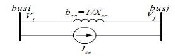
Active and reactive power losses occur in transmission lines depending upon the power to be transmitted. The active power loss equation of the kth line, between buses i and j (fig 2). can be written as (14),

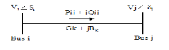
Fig 5.Transmission line
calculated using load flow. If the constraints are
violated, penalty is added to the loss (evaluation value of agent).
Step 3. pbe st is set to each initial searching point. The initial best evaluated value (loss with penalty) among pbe sts is set to gbest.
Step 4. Velocities are calculated using (2).
Step 5. New searching points are calculated using (3).
Step 6. Ploss to the new searching point and the evaluation value is calculated.
Step 7. If the evaluation value of each agent is better than the previous pbest, the value is set to pbest. If the best
pbest is better than gbest, the value is set to gbest. All
of gbe sts are stored as candidates for the final control strategy.
Step 8. If the iteration number reaches to the maximum iteration number, then exit otherwise, go to Step 4.

IJSER © 2011 http://www.ijser.org

International Journal of Scientific & Engineering Research, Volume 2, Issue 2, February-2011 4

ISSN 2229-5518

4.3 VVC Flowchart using PSO

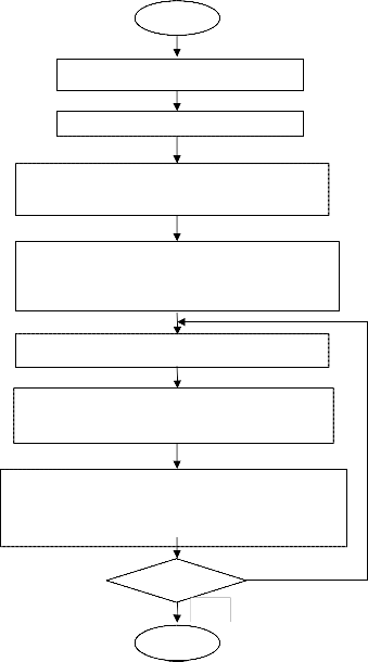
Table -1 Various parameters and their values

Start

Read agents, velocities

Calculate Ploss

If constraint is violated, evaluated value

= Ploss+ Penalty

Set pbest for agent. For best evaluated value, gbest=evaluated value

Calculate velocities and agents

Calculate Ploss and new evaluated value

If new evaluated value is better than pbest, agent= Pbest. For best Pbest, gbest = Pbest and store gbest

5. RESULTS AND DISCUSSION

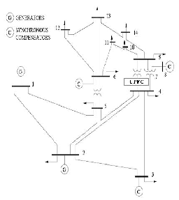
Fig. 7 show the IEEE 14-bus system. UPFC has been included between the buses 4 and 9 in IEEE 14 bus system. Table 2 show the state variables without and with UPFC. Table
3and 4 show power flow results of IEEE 14 bus system without and with UPFC. Table 5 shows the comparative results of proposed system. From the tables it is concluded that the system voltages have been improved and the losses are reduced when UPFC is installed.

If i<n

No

Stop

Yes

4.4 PSO Parameter Control

The following parameters are subjected to vary and their values are given in Table I.

Fig.7 IEEE 14 bus system.

IJSER © 2011 http://www.ijser.org

International Journal of Scientific & Engineering Research, Volume 2, Issue 2, February-2011 5

ISSN 2229-5518

Table -2 State Variables of IEEE 14-Bus System.

.

IJSER © 2011 http://www.ijser.org

International Journal of Scientific & Engineering Research, Volume 2, Issue 2, February-2011 6

ISSN 2229-5518

Table - 3 Power Flows without UPFC.

Table -4 Power Flows with UPFC.

Table 5 Comparative Results.

IJSER © 2011 http://www.ijser.org

International Journal of Scientific & Engineering Research, Volume 2, Issue 2, February-2011 7

ISSN 2229-5518

6. CONCLUSION

This paper presents the application of particle swarm optimization technique in power system state estimation with and without UPFC. The unified power flow controller provides simultaneous or individual controls of basic system parameters like transmission voltage, impedance and phase angle, there by controlling the transmitted power. The Particle Swarm Optimization technique is used to compute the power flow. The power loss occurring in the various branches and state variables of IEEE 5 bus and IEEE 14-bus systems are evaluated using PSO. From the results it is concluded that the system performs better when the UPFC is connected .ie the state variables are improved and the total losses are minimized.

7.REFERENCES

[1] F.C.S.Chweppe,Wildes.i and Rom.d.p, Power System State Estimation part I,II,III, IEEE Transaction on Power Apparatus and System,Januvary1970.
[2] A.Monticelli, Springer-Verlag, State Estimation in Electric Power Systems: A Generalized Approach, (Power Electronics and Power Systems), 1999.
[3] Ali Abur, Garng M. Huang , State Estimation of Power System Embedded with FACTS Devices, Texas A&MUniversity,PSERC Publication 02-45,nov.2002
[4] S. Jshak, A. F. Abidiii and T. K. A. Rahinan Static Var
Compensator Planning Using Artificial Immune System For loss minimization And Voltage Improvement. National Power & Energy Conrerelice (PECon) 2004
[5] L. Gyugyi, T. R. Rietman, and A. Edris, The Unified Power Flow Controller: a New Approach to Power Transmission Control," IEEE Trans. Power Delivery, vol.10, pp. 1085-1092, Apr. 1995.
[6] A. Nabavi_Niaki, and M. R. Iravani, Steady-State and Dynamic
models of Unified Power Flow Controller (UPFC) for Power
System Studies, IEEE Trans. Power Systems, vol. 11, pp. 1937-
1943, Nov. 1996.
[7] S. Tara Kalyani, G. Tulasiram Das, Simulation of Real and
Reactive Power Flow Control with UPFC Connected to a
Transmission Line.Journal of Theoretical and Applied

Information Technology © 2008

[8] Nashiren.F. Mailah , Senan M. Bashi , Single Phase Unified Power Flow Controller (UPFC): Simulation and Construction, European Journal of Scientific Research ISSN 1450-216X Vol.30
No.4 (2009), © EuroJournals Publishing, Inc. 2009
[9] Kennedy and R. Eberhart, Particle Swarm Optimization, Proc. of

IEEE International Conference on Neural Networks, Vol. IV, pp.1942-1948, Perth, Australia,1995

[10] KenichiKawata,Yoshikazu Fukuyama, A Particle Swarm Optimization For Reactive Power and Voltage Control Considering Voltage Stability ,Japan,1999
[11] Z. Huang, Y. Ni, C. M. Shen, F. F. Wu, S.Chen and B. Zang, Application of Unified Power Flow Controller in Interconnected Power System- Modeling, Interface, Control Strategy and Case Study, IEEE Trans. Power Systems, Vol. 15, No. 2, pp. 817-824., May 2000.
[12] D. G. Cho, E. Ho. Song, A Simple UPFC Control Algorithm and Simulation on Stationary Reference Frame,ISIE Conference, Pusan, Korea, pp.1810- 1815, 2001.
[13] Jason Tillett, T.M. Rao, Ferat Sahin and Raghuvee Rao, arwinio

Particle Swarm Optimization ,NY USA

[14] F.G Bagriyanik, Z.E.Aygen and M.BagriyanikPower Loss Minimization Using Fuzzy objective formulation and Genetic Algorithm IEEE power tech Conference, Bolonga, Italy.
[15] N.G.Hingorani, Flexible AC Transmission Systems, IEEE

Spectrum, April 1993, pp. 40–45.

A.S. KANNAN received his B.E degree in Electrical and Electronics Engineering and M.E degree in Power Systems Engineering from Annamalai University, Annamalai Nagar, Chidambaram, India. Currently, he is working as an Assistant Professor in the Department of Electrical and Electronics Engineering, Faculty of Engineering and Technology, Annamalai University, Annamalai Nagar, Chidambaram, India. He has got 11 years of teaching experience. He has attended ten seminars and workshops. His research interests are in Electrical Power Systems, power electronics and FACTs. He is presently pursing Ph.D. in Annamalai University in the Department of Electrical and Electronics Engineering, Annamalai University, Annamalai Nagar, Chidambaram, India.

Email: askannan.aup@gmail.com

Dr. R. KAYALVIZHI received her B.E (Electronics and Instrumentation) and M.E (Power Systems) degrees from Annamalai University with distinction in 1984 and 1888 respectively. She is presently a Professor in the Department of Instrumentation Engineering, Annamalai University where she has put in a total service of 25 years. She has published four national journal papers, four international journal papers, 5 national conference papers and 9 international conference papers. Out of her nine international papers, four papers have been presented in IEEE conferences in Malaysia and Korea. Her research interests are in DCDC converters: modeling, simulation and implementation of intelligent control strategies. She is a life member of Indian society for Technical Education. E-mail: mithuvig.knr@gmail.com

IJSER © 2011 http://www.ijser.org