International Journal of Scientific & Engineering Research Volume 2, Issue 5, May-2011 1

ISSN 2229-5518

Tuning of FOPID Controller Using Taylor

Series Expansion

Ali Akbar Jalali, Shabnam Khosravi

Abstract— In this paper, a direct synthesis approach to fractional order controller design Is investigated. The proposed algorithm makes use of Taylor series of both desired closed-loop and actual closed-loop transfer function which is truncated to the first five terms. FOPID Controller parameters are synthesized in order to match the closed-loop response of the plant to the desired closed-loop response. The standard and stable second-order model is considered for both plant and the desired closed-

loop transfer functions. Therefore for a given plant with damping ratio �1 and natural frequency ron1 . The tuned FOPID controller results in the desired closed-loop response with damping ratio �2 and natural frequency ron2 . An example is presented that

indicates the designed FOPID results in actual closed-loop response very close to desired response rather than PID controller.

It is shown that the proposed method performs better than Genetic Algorithm in obtaining the desired response.

Index Terms— FOPID controller, Taylor series expansion, second order model.

—————————— • ——————————

1 INTRODUCTION

or many decades, proportional-integral-derivative (PID) controllers have been very popular in industries for process control applications. The popularity and
widespread use of PID controllers are attributed primari- ly to their simplicity and performance characteristics. Owing to the paramount importance of PID controllers, continuous efforts are being made to improve their quali- ty and robustness [1], [2].
An elegant way of enhancing the performance of PID controllers is to use fractional order controllers where the integral and derivative operators have non-integer orders. Podlubny proposed the concept of fractional order con- trol in 1999 [3]. In FOPID controller, despite of the pro-
the desired response. The rest of the paper is organized as follows: In section 2 the tuning method for FOPID con- troller is described. An example is investigated in section
3 and finally Section 4 draws some conclusions.

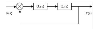
2 OBTAINING THE TUNING METHOD FOR FOPID

CONTROLLER

Consider the block diagram of feedback control system in fig. 1. The objective is design a FOPID controller, Gc (s ), such that for a given plant, G p (s ), with standard second

order model, the actual closed-loop response results in
desired closed-loop response. Desired closed-loop re-
portional, integral and derivative constants, there are two
sponse denoted by

Gd (s ) and described by standard

more adjustable parameters: the power of s in integral and derivative operators, A, )l respectively. Therefore this type of controllers is generalizations of PIDs and conse- quently has a wider scope of design, while retaining the advantages of classical ones.

second order model as follows

ro 2

G d (s ) = n

s 2 H 2�ron s H ro 2

(1)
Several methods have been reported for FOPID design. Vinagre, Podlubny, Dorcak, Feliu [4] proposed a frequen- cy domain approach based on expected crossover fre- quency and phase margin. Petras came up with a method based on the pole distribution of the characteristic equa- tion in the complex plane [5]. In recent years evolutionary algorithms are used for FOPID tuning. YICAO, LIANG, CAO [6], presented optimization of FOPID controller pa- rameters based on Genetic Algorithm. A method based on Particle Swarm Optimization was proposed [7]. In this

Where � , ron

response.

are damping ratio and natural frequency of desired

paper a tuning method for FOPID controller is proposed. Suppose a standard and stable second order plant such that desired response is not available. Tuning FOPID con- troller by the proposed method results in desired closed- loop response. The standard second order is considered for desired response. It is shown that the proposed me- thod performs better than Genetic Algorithm in obtaining

Fig. 1. Block diagram of feedback control system.

According to fig. 1. the actual closed-loop transfer

International Journal of Scientific & Engineering Research Volume 2, Issue 5, May-2011 2

ISSN 2229-5518

function is given by

G (s) = k ( k A( A 1)( A 2)s A 3

Hk )l ()l 1)()l 2)s)l 3 )

(10c)

G s =

G p (s )Gc (s )

(2)

A cl ( )

1 H G p (s )Gc (s )

G ( 4) (s ) = k

( k A ( A 1)( A 2)( A 3)s A 4

In (2), transfer function of FOPID controller is given by

c c i

Hk d )l ()l 1)()l 2)()l 3)s

)l 4 )

(10d)

Gc (s ) = k (1 H

i H k d s

)l )

(3)

(5)

(s ) = k c ( k i A( A 1)( A 2)( A 3)( A 4)s

A 5

(10e)

s A Hk

)l ()l 1)()l 2)()l 3)()l 4)s )l 5 )

Where proportional, integral, derivative constants are
However derivatives of FOPID controller are not de-
denoted by

k c , k i , k d respectively. The orders of integral

fined at s = 0. For convenience and avoiding complexity

and derivative actions, A, ) l , include non-integer values as

that causes by non-integer orders of the Laplace variable s, it is proposed to evaluate (8) and (9) at =1.

0 A, )l 2

(4)
FOPID controller has five tuning parameters. There-
fore five independent equations are needed for tuning
M. Ramasy and Sundaramoorthy in [8] has used dif- ferent structure for FOPID controller as

FOPID controller.

G A cl (1) = G d (1)

(11a)

Gc (s ) = c G c (s )

(5)

G A cl (1) = Gd (1)

(11b)
Where

G (1) = G (1)

(11c)

G (s ) = (s H k i H k s

c s A 1 d

)l H1 )

(6)

A cl d

G A cl (1) = Gd (1)

(11d)

Then for actual closed-loop transfer function in (2), we have

G ( 4) (1) = G ( 4) (1)

G (5) (1) = G (5) (1)

(11e)
(11f)

G A cl (s ) =

k c G p (s )G c (s )

s H k cG p (s )G c (s )

(7)

In obtaining design parameters of FOPID controller, the first terms in (8) and (9) are not considered. According

For designing FOPID controller, it is not possible to set

to (1) and (7),G A cl (s ),G d (s ) are equal in

s = 0. Probably

both

G Acl (s ) and

Gd (s ) equal directly. For each closed-loop

these values are nearly equal in s = 1 . Using (2), the equa-

transfer function, there exist an equal expression but in dif-

ferent structure. This equal expression is Taylor series expan- sion that can be represented for both G Acl (s ) and Gd (s ) in s =

tions in (11) can be written as

G c (1)G p (1) H G c (1)G p (1) G (1) = 0

(12a)

as follows

(s )2 G

( )

(1 H G

c (1)G p

(1))2 d

G A cl (s ) = G A cl ( ) H (s )G A cl ( ) H A cl H ......

(s )2 G ( )

(8)

(Gc (1)G p (1) H 2Gc (1)G p (1) H Gc (1)G p (1))(1 H

Gd (s ) = Gd ( ) H (s )Gd ( ) H d H .......

(9)

G (1)G

(1)) 2(G (1)G

(1) H G (1)G (1))2

2 c p c p c p

G (1) = 0

(12b)

In (8), (9), expressions for derivatives of actual closed-

(1 H Gc (1)G p

(1))3 d

loop transfer function involve derivatives of FOPID control-

(Gc (1)G p (1) H 3Gc (1)G p (1) H 3Gc (1)G p (1) HGc (1)

ler.

G (1))(1 H G (1)G

(1))2 6(G (1)G

(1) H G (1)G (1))

G (s ) = k

( k As A 1 H k

)ls )l 1 )

p c p c p c p

(Gc (1)G p (1) H 2Gc (1)G p H Gc (1)G p )(1 H Gc (1)G p ) H

c c i d

(10a)

6(G (1)G

(1) H G (1)G (1))3 )

G (s ) = k

( k A ( A 1)s A 2 H k

)l ()l 1)s )l 2 )

(10b)

c p c p

(1 H Gc (1)G p

(1))4

Gd (1) = 0

c c i d

(12c)

International Journal of Scientific & Engineering Research Volume 2, Issue 5, May-2011 3

ISSN 2229-5518

(G (4) (1)G

(1) H 4G (1)G

(1) H 6G (1)G

(1)

The nonlinear equations in (12) are complicated to ob-

c p c p c p

tain design parameters, k c , k i , k d , A, )l. thus a nonlinear op-

H4G (1)G

(1) H G (1)G (4) (1))(1 H G (1)G

(1))3

c p c p c p

timization problem must be solved. The fsolve command

6(G (1)G

(1) H 2G (1)G

(1) H G (1)G

(1))2

in optimization toolbox of Matlab is a sufficient tool for

c p c p c p

(1 H G (1)G

(1))2

8(G (1)G

(1) H G (1)G

(1))

solving the set of nonlinear equations. The input argu-

c p c p c p

(Gc (1)G p (1) H 3Gc (1)G p (1) H 3Gc (1)G p (1) H

ments of this command are described as fun, x0 and op- tions. Fsolve starts at an initial value for design parame-

G (1)G

(1))(1 H G (1)G

(1))2 H 36(G (1)G

(1)

ters, x0, in order to solve the set of nonlinear equations

c p c p c p

described in fun. The argument of option determines the

HG (1)G

(1))2 (G (1)G

(1) H 2G (1)G

(1) H G (1)

c p c p c p c

G p (1))(1 H Gc (1)G p (1)) 24(Gc (1)G p (1) H Gc (1)

type of optimization algorithm which is used in solving
the nonlinear equations. The output arguments are the

G (1))4 )

(1 H Gc (1)G p

(1))5

G (4) (1) = 0

(12d)
solution of nonlinear equations, x, and the value of objec-
tive function at x. Consider the nonlinear equations in
(12) as the objective functions. In this case the solution, x,

is the design parameters of FOPID controller, k c , k i , k d , A, )l.

The optimization algorithm of Levenberg-Marquert and

(G (5) (1)G

(1) H 5G (4) (1)G

(1) H 10G

(1)G

(1) H

Gauss-Newton are considered. In the next section, the

c p c p c p

10G (1)G

(1) H 5k G (1)G ( 4) (1) H G (1)G (5) (1))

proposed tuning method is illustrated during an example.

c p c p c p

(1 H G (1)G

(1))4

20(G (1)G

(1) H 2G (1)G

(1)

c p c p c p

HGc (1)G p (1))(Gc (1)G p (1) H 3Gc (1)G p (1) H 3Gc (1)

3 EXAMPLE

In this section, a process from [9] is considered. The ex-

G p (1) H Gc (1)G p (1))(1 H Gc (1)G p (1))

H 90(Gc (1)

ample involves the speed control of a DC motor. Since the

G (1) H 2G (1)G

(1) H G (1)G

(1))2 (G (1)G

(1)

most basic requirement of a motor is that it should rotate

p c p c p c p

at the desired speed, the steady-state error of the motor

HG (1)G

(1))(1 H G (1)G

(1))2

10(G (1)G

(1)

c p c p c p

speed should be less than 1%. We want to have settling

HG (1)G

(1))(G ( 4) (1)G

(1) H 4G (1))G

(1) H 6

time of 2s and an overshoot of 4%. A desired closed-loop

c p c p c p

(4)

transfer function that includes all of the design specifica-

Gc (1)G p (1) H 4Gc (1)G p (1) H Gc (1)G p

(1))(1 H Gc (1)

tions, can be defined as follows

G (1))3 H 60(G

(1)G

(1) H G (1)G

(1))2 (G (1)G

(1)

p c p c p c p

H3k cGc (1)G p (1) H 3Gc (1) G p (1) H Gc (1)G p (1))(1 H

G (s ) = 8.9401

d s 2 H 4.2398s H 8.9401

(14)

G (1)G

(1))2

240(G (1)G

(1) H G (1)G

(1))3 (G (1)

c p c p c p c

G p (1) H 2Gc (1)G p (1) H Gc (1)G p (1))(1 H Gc (1)G p (1)) H

The transfer function of the process is defined by

120(G (1)G

(1) H G (1)G

(1))5

c p c p

(1 H Gc (1)G p

(1))6

G (5) (1) = 0

(12e)

G p (s ) = 0.0999 2

20.02

H 12s H 20.02

(15)
Applying the values of

G (1),G

(1),G

(1),G ( 4) (1)

Where

G (5) (1),G

(1),G

p p p p p

(1),G (4) (1),G (5) (1) in (12), five nonli-

Gc (1) = k c (1 H k i H k d )

(13a)

p d d d d d d

near equations are obtained. Using the fsolve command
in optimization toolbox of Matlab, the fractional order
controller is designed as

Gc (1) = k c (

k i A H k d )l )

(13b)

G (s ) = 18.27(1 H 1.11

0.563s 0.1)

(16)

Gc (1) = k c (

k i A ( A

1) H k d )l () l 1))

(13c)

c s 1.02

After designing the FOPID controller, the values of

Gc (1) = k c (

k i A ( A

1)( A

2) H k d )l ()l

1)()l

2))

(13d)
nonlinear equations in (12), are

10 4 , 10 4 , 10 4 , 10 4 ,10 3.

It is obvious that the obtained values for design parame-

G ( 4) (1) = k

( k A ( A

1)( A

2)( A

3) H k

)l () l 1)

ters, k , k , k

, A, )l. , are very close to roots of nonlinear eq-

c c i d

(13e)

c i d

()l

2)()l

3))

uations in (12). Furthermore the values of both actual and
desired closed-loop transfer functions at s = 1 are nearly

10 3 . Thus the first six terms of

G (5) (1) = k (

k A ( A

1)( A

2)( A

3)( A 4)

equal with difference of

c c i

(13f)
Taylor series of actual closed-loop transfer function are

H k d )l ()l

1)( )l

2)()l

3)()l

4))

equal to same order terms for desired one. The accuracy of how much the actual closed-loop response is close to

International Journal of Scientific & Engineering Research Volume 2, Issue 5, May-2011 4

ISSN 2229-5518

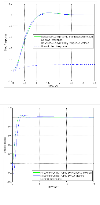
desired response can be concluded from fig. 2. For com- parison, the tuned FOPID controller using Genetic Algo- rithm is considered. Fig. 3 shows that the closed-loop re-

TABLE 1

SPECIFICATIONS OF DESIRED CLOSED-LOOP RESPONSE

sponse under FOPID controller, which is tuned by both GA and proposed methods, in comparison to desired re- sponse. Data about specifications of desired closed-loop

Maximum

overshoot

Settling

time

Rise time Steady-

state error

response are collected in Table1.

4 2 0.9 0

Table. 1. reports the maximum overshoot (in %), set- tling time and rise time (in second) and steady-state error (in %) for the closed-loop step response. Data about the performance of closed-loop system under FOPID and PID controllers against unit step, are collected in Table 2.

TABLE 2

SUMMERY OF THE PERFORMANCE OF CLOSED-LOOP SYSTEM UNDER FOPID AND PID CONTROLLER AGAINST UNIT STEP

Different controllers

Maximum overshoot

Settling time

Rise time Steady- state

error

Fig. 2. Step response of closed-loop system using both FOPID and PID controllers, step response of the desired closed-loop system, step response of uncontrolled system.

FOPID using proposed method

FOPID using GA method PID using proposed

4 2.08 0.9 0

4.5 5.3 1.26 0

2 1.08 0.86 0

method

Fig. 3. Step response of closed-loop system using FOPID control- ler obtained by proposed method and Genetic Algorithm tuning method, step response of the desired closed-loop system.

Fig. 2. compares actual closed-loop response under both PID and FOPID controllers and desired response. In fig. 2. PID and FOPID controllers are tuned by proposed method. Due to Table. 2. the actual closed-loop response under FOPID controller is very close to desired response rather than applying PID controller. For example the spe- cifications of transient response, such as maximum over- shoot, rise time, settling time and steady-state error when using FOPID controller, are very close to desired transient specifications. Using PID controller results in a behavior in t=0, which is not appeared when applying FOPID con- troller. This behavior is because of existing a zero near the origin. Furthermore due to fig.3. and Table. 2 the FOPID controller, which is tuned by proposed method, results in better performance rather than FOPID controller which is tuned by GA method.
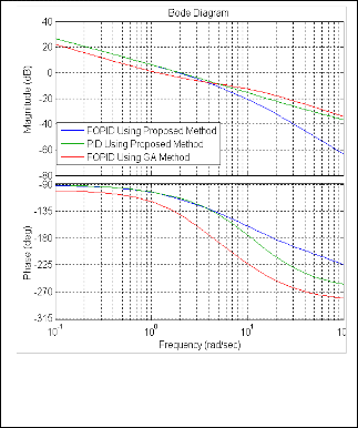
Fig. 4. shows the bode diagram of open-loop systems, applying both FOPID and PID controllers.

International Journal of Scientific & Engineering Research Volume 2, Issue 5, May-2011 5

ISSN 2229-5518

REFERENCES

[1] Y.X. Su, Dong Sun, B.Y. Duan, "Design of an enhanced nonlinear PID controller", Mechatronics, Vol 15, No. 8, pp. 1005–1024, Oc- tober 2005.

[2] Deepyaman Maiti, Ayan Acharya, Mithun Chakraborty, Amit Konar,

Ramadoss Janarthanan, "Tuning PID and

PI A D )l Controllers using

Fig. 4. Bode diagram of open-loop systems applying FOPID contro ler which is tuned by both proposed method and GA method, bod diagram of open-loop system applying PID controller which is tuned by proposed method.

According to fig.4. applying FOPID and PID control- lers which is tuned by proposed method result in a same phase margin of 66 (deg). However the difference in val- ues of gain margin is significant. The gain margin of 30.7 (dB) and 17(dB) are obtained for FOPID and PID control- lers respectively. The FOPID controller which is tuned by Genetic Algorithm results in gain margin and phase mar-

the Integral Time Absolute Error Criterion", 4th IEEE International Conference on Information and Automation for Sustainability, Nov 2008.

[3] Igor Podlubny, "Fractional-order systems and PI A D )l controllers",

IEEE Transactions on Automatic Control, Vol 44, No. 1, pp.

208–213, JANUARY 1999.

[4] Vinagre, B.M., Podlubny, I., Dorcak, L., Feliu, V., 2000. "On frac- tional PID controllers: a frequency domain approach". In: Proceed- ings of IFAC Workshop on Digital Control-PID, 2000, Terrassa, Spain.

[5] Petras, I., 1999. "The fractional order controllers: methods for their synthesis and application". Journal of Electrical Engineering 50 (9–10), 284–288, Apr 2000.

[6] JUN-YICAO, JIN LIANG, BING-GANG CAO, "optimization of fractional order PID controllers based on genetic algorithms", pro- ceeding of fourth International Conference on Machine Learn- ing and Cybernetics, Guangzhou, Vol 9, pp. 5686-5689, 18-21

August 2005.

[7] Deepyaman Maiti, Sagnik Biswas, Amit Konar, "Design of a Fractional Order PID Controller UsingParticle Swarm Optimization Technique", 2nd National Conference on Recent Trends in In- formation Systems Oct 2008.

[8] M. Ramasamya, S. Sundaramoorthy, "PID controller tuning for

desired closed-loop responses for SISO systems using impulse re- sponse", Computers and Chemical Engineering 32 (2008) 1773–

1788.

[9] Arijit Biswas, Swagatam Das, Ajith Abraham, Sambarta Das-

gin of 8.2(dB) and 59 (deg) respectively. It can be con-

A )l

gupta, "Design of fractional-order PI D

controllers with an im-

cluded that better performances can be obtained by using the proposed method.

4 CONCLUSION

A design method for FOPID controller is proposed. This method is based on Taylor series of both actual and desired closed-loop transfer function. The design parame- ters of controller are used for matching the same order terms of both desired and actual closed-loop response. FOPID controller has two design parameters, A, )l , more than PID controller. Thus two more terms in Taylor series are used to match closed-loop response to desired re- sponse. This causes increasing accuracy in tracking the desired response rather than using PID controller. Fur- thermore the FOPID controller which is tuned by pro- posed method performs better than FOPID controller which is tuned by Genetic Algorithm. It can be concluded that that better performances can be obtained by the pro- posed method.

proved differential evolution", Enginnering Application of Artifi-

cial Intelligence, Vol 22, No. 2, pp. 343-350, March 2009.