International Journal of Scientific & Engineering Research Volume 4, Issue 2, February-2013 1
ISSN 2229-5518
Theoretical Study Of Heat Transfer In Circular
![]()
Holes For Turbine Blade
* AL-Nahrain University, College of Engineering, Jadiriya, P.O. Box 64040, Baghdad, Iraq
ABSTRACT— Turbine airfoils are exposed to the hott est temperatures in the gas turbine with tem peratures typically exceeding the melting point of the blade mat erial. Cooling methods investigated in this com putational study included parasitic cooling flow losses, which are inherent to engines. Film-cooling is one typically used cooling m ethod whereby coolant is supplied through holes placed along the camber line of the blade.
The subject of this paper is to evaluat e the heat transfer that occur on the holes of blade through different blowing ratio from at (05%, 1%, 1.5% and
2%). The cases of this study were performed in a low speed wind tunnel and m ultiple coolant flow rates through the film-cooling holes. A range of blowing ratios (U∞/Uc) was studied whereby coolant was injected from holes placed along the camber line of the blade with a large scale blade model with the mainstream velocity at 11.3 m/s. Numerical was conducted in a linear cascade with a scaled-up turbine blade whereby the Reynolds
number of the engine was matched (2.1*105). Overall, the holes appears to be a feasible m ethod for prolonging blade life.
Keywords: blade cooling, CFD, gas turbine, heat transfer, mass transfer.
—————————— ——————————
as turbine engines are widely used to power aircraft because they are light and compact and have a high power to- weight ratio. One way to increase power and efficiency of gas turbines is by increasing turbine-operating temperatures. The motivation behind this is that higher temperature gases yield higher energy potential. However, the components along the hot gas path experience high thermal loading, which can cause distress. The HPT (High
Pressure Turbine) first stage blade is one component that is extremely vulnerable to the hot gas.
The two main objectives of blade design engineers are (1) to reduce the leakage flow either by reducing the tip gap or by implementing a more effective tip leakage sealing mechanism and (2) to cool the blade tips with the least possible usage of cooling fluid.
The degree of cooling which may be achieved is dependent upon a number of factors, chief among which are (a) the temperature difference between the main gas stream and the inlet cooling air and (b) the 'conductance ratio', this being defined as the ratio of the heat input to the blade per unit temperature difference between gas stream and blade to the heat passed to the cooling air per unit temperature difference between blade and cooling air (viz. hgSg/hcSc).
Clearly to achieve a high degree of cooling the lowest possible value of conductance ratio is required in conjunction with the largest possible temperature difference between gas stream and cooling air. The heat input to the blade per unit temperature difference between gas stream and blade is the product of the average gas-to-blade heat transfer coefficient and the external surface area, and this in turn is dependent upon the blade shape, gas flow incidence, gas flow Reynolds number, gas Prandtl number, and to a lesser extent upon the ratio of gas temperature to blade temperature, and also gas stream Mach number,[1].
The cooling air is forced through a porous blade wall. This method is by far the most economical in cooling air, because
not only it remove heat from the wall more uniformily, but the effuission layer of air insulates the outer surface from the hot gas stream and so reduces the rate of heat transfer to the blade,[2].
In present study, the mainstream temperature (Tg) that used to heat the blade at 750 C (take from al-Dorah power station) and the temperature of coolant flow (Tc) at 27 C and the pressure at atmosphere condition. And numbers of holes that used in this syudy is ten holes.
The work presented in this paper is concerned with the effects of injecting coolant to the tip of a turbine blade, where the experiments were completed for a stationary, linear cascade. As such, it is important to consider the relevance of past studies to evaluate the effects of the relative motion between the blade tip and outer shroud. It is also relevant to consider tests where tip blowing has been investigated.
Allen and Kofskey (1955) [3], performed some visualization teats to see what these secondary flows looked like. Additionally, they also studied the effect of ejecting flow from the turbine tips on the shape of the secondary flows. At the time of these tests, engine temperatures were not so high as to require cooling of the turbine blades for operation but they noted that, "turbine blade cooling may become an engine requisite. The turbine rotor blade cooling method of passing cooling air through hollow blades and discharging it at the blade tip may be one of the most feasible methods of changing the secondary-flow pattern".
Yang et al. (2004) [4] predicted film cooling effectiveness and heat transfer coefficient for three types of film-hole arrangements: 1) the holes located on the mid-camber line of the tips, 2) the holes located upstream of the tip leakage flow and high heat transfer region, 3) combined arrangements of camber and upstream holes. They found
IJSER © 2013 http://www.ijser.org
International Journal of Scientific & Engineering Research Volume 4, Issue 2, February-2013 2
ISSN 2229-5518
that upstream film hole arrangements provided better film cooling performance than camber arrangements.
Acharya et al. (2003) [5] indicated that film cooling injection lowered the local pressure ratio and altered the nature of the leakage vortex. High film-adiabatic effectiveness and low heat transfer coefficients were predicted along the coolant trajectory with the lateral spreading of the coolant jets being quite small for all cases. With an increased tip gap the coolant was able to provide better downstream effectiveness through increased mixing. For the smallest tip gap, the coolant was shown to impinge directly on the surface of the shroud leading to high film effectiveness at the impingement point. As the gap size increased, their predictions indicated that the coolant jets were unable to penetrate to the shroud
Nasir et al. (2003) [6] again found that a single squealer on the suction side performed the test. The performance of different recessed tip geometries were investigated and compared with plane tip performance. A transient liquid crystal technique was employed to measure detailed heat transfer coefficient distributions. Coolant injection from holes located on the blade tip, near the tip along the pressure side and combination cases were also investigated. Experiments were performed for plane tip and squealer tip for different coolant to mainstream blowing ratios of 1.0,
2.0, and 3.0. A transient infrared (IR) thermography technique was used to simultaneously measure heat transfer coefficient and film cooling effectiveness. He shows the tip
injection reduced heat transfer coefficient on the blade tip and an increase in blowing ratio caused a decrease in heat transfer coefficient for both plane and squealer tip blade.
Christophel et al. (2004a) [7] evaluated the adiabatic effectiveness levels that occur on the blade tip through blowing coolant from holes placed near the tip of a blade along the pressure side. A range of blowing ratios was studied where by coolant was injected from holes placed along the pressure side tip of a large scale blade model. Also present were dirt purge holes on the blade tip, which is part of a commonly used blade design to expel any large particles present in the coolant stream. Experiments were conducted in a linear cascade with a scaled-up turbine blade where by the Reynolds number of the engine was matched, from these tests indicated that the performance of cooling holes placed along the pressure side tip was better for a small tip gap than for a large tip gap. Disregarding the area cooled by the dirt purge holes, for a small tip gap the cooling holes provided relatively good coverage. For all of the cases considered, the cooling pattern was quite streaky in nature, indicating very little spreading of the jets. As the blowing ratio was increased for the small tip gap, there was
most microcircuit film-cooling cases. Significant leading edge cooling was obtained from coolant exiting from dirt purge holes with a small tip gap while little cooling was seen with a large tip gap. Also the migration of coolant from the front leakage was shown to cool a considerable part of the platform. Several hot spots were predicted along the platform, which were circumvented through the placement of microcircuit channels. Ingestion of hot mainstream gas was predicted along the aft portion of the gutter and agreed with distress exhibited by actual gas turbine engines.
Couch (2003) [9] studied examinations of a novel cooling technique called a microcircuit, which combines internal convection and pressure side injection on a turbine blade tip. Holes on the tip called dirt purge holes expel dirt from the blade, so other holes are not clogged. Wind tunnel tests were used to observe how effectively dirt purge and microcircuit designs cool the tip. Tip gap size and blowing ratio are varied for different tip cooling configurations. Results show that the dirt purge holes provide significant film cooling on the leading edge with a small tip gap. Coolant injected from these holes impacts the shroud and floods the tip gap reducing tip leakage flow. Also, results suggest that blowing from the microcircuit diminishes the tip leakage vortex. Overall, the microcircuit appears to be a feasible method for prolonging blade life.
In summary, The objectives of the work presented in this paper are to present the benefits of heat transfer of a holes using coolant exhausted from holes to tip. In particular, both the effectiveness levels and heat transfer coefficients were calculated
The basic equations that describe the flow and heat are Conservation of Mass, momentum and energy equations. These equations describe two-dimensional, turbulent and incompressible flow takes which the following forms (Arnal, M.P,1982)[10]:
The assumptions that used for the instantaneous equation are:-
1- Steady, two-dimensional, incompressible flow, adiabatic, single phase flow, shock free, inviscous, no slip, irrotational.
2- The fluid is Newtonian.
3- Cylinderical coordinate.
![]()
![]()
a (pu) + 1 a (ρrv) = 0 … (1)
an increase in the local effectiveness levels resulting in az
higher maxima and minima of effectiveness along the
r ar
middle of the blade.
Hohlfeld et al. (2003) [8] investigated in this computational
u-momentum (z-direction)
study included parasitic cooling flow losses, which are 1 a a
a 1 a
au a
inherent to engines, and microcircuit channels. This study![]()
![]()
![]()
![]()
![]()
![]()
![]()
![]()
[ (ρruu) + (ρruv) ]= − + [ (rJ- ) +
r az ar az r az az ar
![]()
au
evaluated the benefit of external film-cooling flow
exhausted from strategically placed microcircuits. Along the
(rJ-eff
)] + Su … (2)
ar
blade tip, predictions showed mid-chord cooling was
independent of the blowing from microcircuit exits. The
formation of a pressure side vortex was found to develop for
v-momentum (r-direction)
IJSER © 2013 http://www.ijser.org
International Journal of Scientific & Engineering Research Volume 4, Issue 2, February-2013 3
ISSN 2229-5518
![]()
![]()
![]()
![]()
![]()
![]()
1 [ a (ρruv) + a (ρrvv) ]=- ap + 1 [ a (rμ
![]()
![]()
av ) + a (rμ
a v
where :-
r az ar
ar r az
eff az
ar eff ar
) - Γv v ]+ S
… (3)![]()
r2 v
(ø) is any dependent variable.
( ø) is any exchange coefficient of ø.
![]()
![]()
![]()
![]()
![]()
1 [ a (ρruT) + a (ρrvT) ]= 1 [ a (rr![]()
![]()
ar ) + a (rr![]()
ar )]
(Sø) is the source term of ø.
r az ar
r az
eff az
ar eff ar
The transform equation (10) from physical domain
… (4)
The turbulence model utilized in this analysis is the two
to computational domain, and that lead to obtained the transformation of the governing equations as follows:-
equation k-Epsilon model. This model is utilized for its a
a a aø a aø
proven accuracy in turbine blade analysis and for its applicability to confined fluid flow. ( k- ε) Turbulence Model is one of the most widely used turbulence models is the two-equation model of kinetic energy (k) and its dissipation rate (ε). The turbulence according to Launder and Spalding [11] is assumed to be characterized by its kinetic energy and dissipation rate (ε), where
![]()
![]()
![]()
![]()
![]()
![]()
(ρøG1) + (ρøG2) = rø ]a + rø ]c + Stotal
a( a1 a( a( a1 a1
… (11)
where:-
G1 and G2 are the contravariant velocities or the mass flow rates in the ζ and η direction respectively.
The governing equations are integrated over each control volume (C.V.) with each its neighbor nodes. This![]()
![]()
1 a
[
r az
![]()
a
(ρruk) +
ar
![]()
1
(ρrvk) ] =
r
![]()
![]()
[ a (rrk ) + a
az az ar
(rrk + G
ar
discretization of the steady, 2-D governing equations is done
+ Gb – ρε – YM … (5)
1 [ a (ρruε) + a (ρrvε) ] = 1 [ a (rr E aε )+ a (rr E aε )] + c
by using finite volume method with collocated grid
arrangement by using the upwind differencing scheme. Also discretization the terms of source term to give the solving
the governing equations.![]()
![]()
![]()
![]()
![]()
![]()
![]()
![]()
r az
ε
ar
![]()
![]()
![]()
ε2 E
r az
az ar ar 1
After solving the momentum equation, the velocity field
G - c2 ρ + k
C1C2Gb … (6)
obtained does not guarantee the conservation of mass unless
the pressure field is correct, therefore, the velocity
where
a u 2
a v 2 v 2
a u
a v 2
component (u, v), (G1,G2), pressure must be corrected
according to the continuity equation, (Karki and Patankar,
1989)[13].
G = J-t {2[(az )![]()
+ (ar )
+ ( ] + ( } + S
r az ar
… (7)
In the present work, the (SIMPLE) algorithm (Semi-Implicit Method for Pressure Linked Equation) is used to couple the pressure and velocity as in (Veresteeg & Malalasekera,
SG given by ( Ideriah, F. J. K.,1975)[12]
1995)[14]. This method is done by solving the momentum equations using the guessed pressure field to obtain the
2 au
av 2 2
au av
velocity then, the velocity field that obtained satisfies the![]()
![]()
![]()
![]()
![]()
![]()
SG = - 3 J-t az + ar - 3 ρk az + ar … (8)![]()
2 Ek
momentum equations, then the velocity and pressure are corrected because the velocity field violates the conservation
Also, Y =
a2
, The compressibility modification always
of mass.
takes effect when the compressible form of the ideal gas low
is used, but in present work is take the flow in a incompressible. Additionally, since gravity is neglected the contribution of buoyancy (Gb) to the turbulence transport equations is also neglected.
also, J-t = ρcf1 k2 / ε … (9)
The values of the empirical constant used here are given in
Table (1). (Launder and Spalding,1974) [11].
Cμ | CD | C1 | C2 | σk | σε |
0.09 | 1.0 | 1.44 | 1.92 | 1.0 | 1.3 |
The governing equations (1),(2),(3),(4),(5) and (6) can be write in one general form as shown below:
To better understand the effects of the heat transfer in holes, a computational fluid dynamics (CFD) simulation was also performed. A commercially available CFD code, Fluent
6.3.26 [15] was used to perform all simulations. Fluent is a pressure based flow solver that can be used with structured or unstructured grids. An unstructured grid was used for the study presented in this paper. Solutions were obtained by numerically solving the Navier-Stokes and energy equation through a control volume technique. All geometric construction and meshing were performed with GAMBIT
2.4.6. To ensure a high quality mesh, the flow passage was
divided into multiple volumes, which allowed for more control during meshing. The tip gap region was of primary concern and was composed entirely of tetrahedral cells with an aspect ratio smaller than three.
Inlet conditions to the model were set as a uniform inlet velocity at approximately one chord upstream of the blade.![]()
a( uø) + 1 a( rvø ) = a ( ø aø )+ 1 a (r ø aø )+S
… (10)![]()
![]()
![]()
![]()
![]()
az r ar
az az
r ar
ar ø
IJSER © 2013 http://www.ijser.org
International Journal of Scientific & Engineering Research Volume 4, Issue 2, February-2013 4
ISSN 2229-5518
Figure (1) shows the mesh of the test rig. An inlet mass flow boundary condition was imposed for the coolant at the plenum entrance for the cooling holes.
The mesh contained approximately 20 grid points across the hole exit. Mainstream flow angles were set to those of the experiments as well as the scaled values for the engine while the turbulence levels and mixing length were set to
1% and 0.1 m, respectively.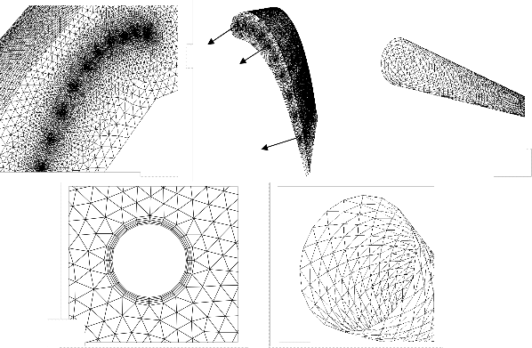
Computations were also performed with an inlet turbulence level of 10%, but no noticeable differences were predicted between the 1% and 10% inlet turbulence casesAll other experimental conditions were matched in the simulations including the temperature levels and flow rates. To allow for
reasonable computational times, all computations were performed using the RNG k-ε turbulence model with non- equilibrium wall functions whereby the near wall region was resolved to y+ values ranging between 30 and 60. Mesh insensitivity was confirmed through several grid adaptions based on viscous wall values, velocity gradients, and temperature gradients. Typical mesh sizes were composed of 4.8 million cells with 40% of the cells in and around the tip gap region. Typical computations required 2000 iterations for convergence.
1
5
10 (a)
(b)
(c)
(d)
(e)
Next the average heat transfer coefficient for the cold side is
In the present study, is to use the calculated mass flow rates and fluid exit temperatures for all cooling holes to calculate the total heat :
Q= ṁ Cp (Te –T in) … (12) Where Tin is cold temperature.
After that comparing between total heat transfer with heat transfer by convection in holes to find heat transfer coefficient, when the last is use to calculate nusselt number for different wall temperature around the pipe.
h d
found by averaging the heat transfer coefficients predicted by Dittus-Boelter correlation for each hole:
Nu = 0.023 (Re pipe)n (Pr)s … (14) Where n=0,8, s= 0.4 (heating flow)
Results are shown for cases with a baseline flat tip and coolant injection at a small and large tip gap (0.003 and
0.009m) respectively. Blowing ratios of 0.5%, 1%, 1.5%
and 2% of the core inlet flow to explore thermal and flow![]()
Nux =
k
… (13)
effects within the passage. The results are presented in the dimensionless form of static pressure coefficient and adiabatic effectiveness.
IJSER © 2013 http://www.ijser.org
International Journal of Scientific & Engineering Research Volume 4, Issue 2, February-2013 5
ISSN 2229-5518
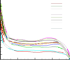
at midspan for small tip gap in suction and pressure side with the pressure non-dimensionalized by the inlet pressure conditions and given in Cp parameters. Also this results comparison with experimental and computational data for Christophel et al (2005a)[38]. When the air approaching the leading edge of a blade is first slowed down, it then speeds up again as it passes over or beneath the blade. As the velocity changes, so does the dynamic pressure and static
pressure according to Bernoulli's principle. Air near the stagnation point has slowed down, and thus the static pressure in this region is higher than the inlet static pressure to main duct. Air that is passing above and below the blade, and thus has speeded up to a value higher than the main inlet path velocity, will produce static pressures that are lower than inlet static pressure. At a point near maximum![]()
520
500
480
460
440
420
400
380
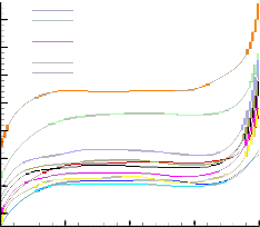
hole 1 hole 2 hole 3 hole 4 hole 5 hole 6 hole 7 hole 8 hole 9 hole 10
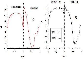
thickness, maximum velocity and minimum static pressure will occur. Also this figure shows a good agreement with the experimental and computational data for Christophel et al..
0 0.25 0.5 0.75 1
z/s
![]()
![]()
![]()
0.9
0.85
0.8
0.75
0.7
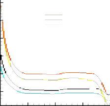
hole 1 hole 2 hole 3 hole 4 hole 5 hole 6 hole 7 hole 8 hole 9 hole 10
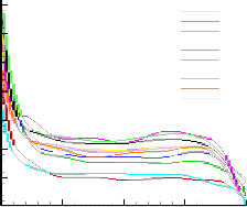
shows the low temperature at hole 3 and hole 4 becouse maxiumim distance between suction and pressure and the high temperature at the surface is not affect largely to this holes. From Figure (3), the wall temperature has minumim value (temperature of air) at zero dimensional horizontal Z, and maximum value at the end of dimensional distance because the mixing between cooled and high temperature.
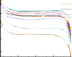
0.2 to o.85, and degreases at the end of dimensionless, because the large temperature difference between the flow
and wall. Addisionaly heat transfer coefficient at zero dimensionless is very large.
IJSER © 2013 http://www.ijser.org
International Journal of Scientific & Engineering Research Volume 4, Issue 2, February-2013 6
ISSN 2229-5518
225
200
175
150
125
hole 1 hole 2 hole 3 hole 4 hole 5 hole 6 hole 7 hole 8 hole 9 hole 10
4
3.5
3
2.5
2
hole 1 hole 2 hole 3 hole 4 hole 5 hole 6 hole 7 hole 8 hole 9 hole 10
100
1.5
75 1
50
0 0.25 0.5 0.75 1
Z/S
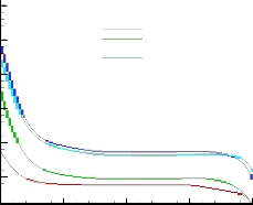
0.85 of dimensionless and decrease at the end of dimensionless. Also, the hole 1 and hole 10 have minimum
nusselt numder and hole 5 has maximum nusslelt number. Also Figure (7) show the dimensionless nusselt number relate with dimensionless distance of span.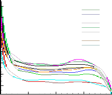
45 hole 1 hole 2 hole 3
40 hole 4
hole 5
35 hole 6 hole 7
hole 8
30 hole 9
hole 10
25
20
15
10
0 0.25 0.5 0.75 1
Z/S
0 0.25 0.5 0.75 1
Z/S
All Figures take at small tip gap with blowing ratio at (1%), but in large tip gap is not different large in small tip gap only at exit of holes in the tip.
IJSER © 2013 http://www.ijser.org
International Journal of Scientific & Engineering Research Volume 4, Issue 2, February-2013 7
ISSN 2229-5518
Pwr,Coef
E+0013.628998499133
35 E+0022.593190373882-
E+0027.197597391923
E+0037.818425288480
30 E+0047.735443350674-
E+0053.153651557898
25 E+0057.322910434303-
E+0061.035228374508
E+0058.821576087699-
20 E+0054.168123534584
E+0048.391007002910-
15
| 0
| 1
| 2
| 3
| 4
| 5
| 6
| 7
| 8
| 9
| 10
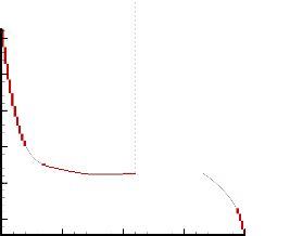
1.5% and 2% are lowest values of dimensionless Nusselt number of low blowing ratios at 0.5% and 1%, because the coolant flow impacts the shroud and makes the flow inside pipe slow, and notes the coolant flow is poor mixed with the leakage flow, therefore that makes the high blowing ratio decrease.
10
0 0.25 0.5 0.75 1
z/s
3.5
3
2.5
0.5% Blowing at hole 4
1% Blowing at hole 4
1.5% Blowing at hole 4
2% Blowing at hole 4
2
3.5
3
2.5
0.5% Blowing at hole 1
1% Blowing at hole 1
1.5 % Blowing at hole 1
2 % Blowing at hole 1
1.5
1
2
1.5
1
0 0.25 0.5 0.75 1
z/s
0 0.25 0.5 0.75 1
z/s
From the results, it can be concluded that the heat transfer has the maximum value can be reached at the hole of the number 4. Also heat transfer results on the holes shows when changing the blowing ratio of 1.5% (the maxing
Symbol Description Dimension
A Coefficient of the discretized m2
equation, area
Bx Axial Chord of the blade m
C Chord of the blade m
change) in (Nux/Nu) than 2%, 1%, 0.5% respectively. Heat
transfer coefficient is high values at entrance regions.
Results showed that baseline Nusselt numbers on the holes were reduced along the holes. Also results indicated the amount of cooling that used to cooled the blade is limited.
J Jacobian of coordinates pa transformation
P pressure m
Repipe Reynolds Number (Re=ρUD/μ) k
S Span length m/sec
Sɸ Source term of ɸ - T Temperature C
G1,G2 Contravariant velocity in ξ,η,ζ
respectively
m/sec
u ,v Velocity component in z, r
respectively -
IJSER © 2013 http://www.ijser.org
International Journal of Scientific & Engineering Research Volume 4, Issue 2, February-2013 8
ISSN 2229-5518
P Static pressure N/m2
Tg Temperature of hot gases C
Tc Temperature of cooling air C
ɸ Dependent variable
η Adiabatic effectiveness ,η= (Tin- Taw)/(Tin-Tc)
u, v Velocity component in z ,r coordinate direction respectively
r,z Cylinderical coordinate
m/sec
Cp (( − ( n )/(0.5 p U2 )
ρ Density Kg/m3
N/m2
ε Rate of dissipation of kinetic energy
m2/sec-3
ζ,η partial derivative in the
computational plane -
c Coolant conditions -
∞ Mainstream conditions
-
[1] Jonas B., "Internal cooling of gas turbine blades", 2000. [2] Cohen H., Rogers G.F.C., and Saravanamutto H.I.H.,
"Gas turbine theory", 3rd edition, Longman scientific and technical, 1987.
[3] Allen, H. W. and M.G. Kofskey, "Visualization Study of Secondary Flows in Turbine Rotor Tip Regions", NACA Technical Note 3519, 1955.
[4] Yang Huitao, Hamn-Ching Chen and Je-Chin Han, "Numerical Prediction of Film Cooling and Heat Transfer With Different Hole Arrangements on the plane and Squealer Tip of a Gas Turbine Blade", ASME Paper No. GT2004-53199, 2004.
[5] Acharya, S., H. Yonk, C. Prakash and R. Bunker, "Numerical Study of Flow and Heat Transfer on a Blade tip with Different Leakage Reduction Strategies'', ASME paper No. GT-2003-38617, 2003.
[6] Nasir Hasan Srinath, V. Ekkad, Divad M. Kontrovitz, Ronald S. Bunker and Chander prakash, "Effect of Tip Gap and Squealer Geometry on Measured Heat Transfer Over a HPT Rotor Blade Tip", J. of Turbomachinery, 125, pp. 221-
228, 2003.
[7] Christophel, J. R., E. Couch, K. A. Thole and F. J. Cunha, "Measured Adiabatic Effectiveness and Heat Transfer for Blowing from the Tip of a Turbine Blade", ASME paper No. GT2004-53250, 2004.
Tip and Platform of a Turbine Blade", Master's Thesis,
µ Dynamic viscosity N.m/Sec2
C.F.D Computational Fluid Dynamics
2D Two-Dimensional
SIMPLE Semi-Implicit Method for
Pressure Linked Equation
RANS Reynolds-averaged Navier- Stokes
Virginia Polytechnic Institute and State University, Blacksburg, VA, 2003.
[9] Couch, E., "Measurement of Cooling Effectiveness along the Tip of a Turbine Blade", Master's Thesis, Virginia Polytechnic Institute and State University, Blacksburg, VA,
2003.
[10] Arnal, M.P., "A General computer program for two- dimensional, turbulent, re-circulating flows", Report No.Fm-83-2, 1983.
[11] Launder, B.E. and Spalding, D.B.," Mathematical models of turbulence", Academic press, London, 1972.
TEACH", private communication, 1975
1167-1174, 1989,
IJSER © 2013 http://www.ijser.org