International Journal of Scientific & Engineering Research, Volume 3, Issue 7, July-2012
ISSN 2229-5518
The effect of probabilities of departure with time in a bank
Kasturi Nirmala, Shahnaz Bathul
Abstract— This paper deals with the Queueing theory and analysis of probability curves of pure death model. Starting with the historica l back grounds and important concepts of Queueing theory, we obtained a relation to find time “t” where we get highest probabil ity for departures which follow truncated Poisson probability distribution.
Poisson probability distribution
—————————— ——————————
lot of our time is consumed by unproductive activities. Tra- velling has its own demerits one of them being wastage of time getting caught in traffic jams. A visit to the Post office or bank is very time consuming as huge crowds are waiting to be serviced. A simple shopping chore to a supermarket leads us to face long queues. In general we do not like to wait.
People who are giving us service also do not like these delays
because of loss of their business. These waits are happening due to the lack of service facility. To provide a solution to these problems we analyze queueing systems to understand the size of the queue, behavior of the customers in the queue, system capacity, arrival process, service availability, service process in the system. After analyzing the queueing system we can give suggestions to management to take good deci- sions.
A queue is a waiting line. Queueing theory is mathematical theory of waiting lines. The customers arriving at a queue
may be calls, messages, persons, machines, tasks etc. we iden-
tify the unit demanding service, whether it is human or oth- erwise, as a customer. The unit providing service is known as server. For example (1) vehicles requiring service wait for their turn in a service center. (2) Patients arrive at a hospital for treatment. (3) Shoppers are face with long billing queues in super markets. (4) Passengers exhaust a lot of time from
the time they enter the airport starting with baggage, security
checks and boarding.
Queueing theory studies arrival process in to the system, waiting time in the queue, waiting time in the system and service process. And in general we observe the following type of behavior with the customer in the queue. They are Balking of Queue:
————————————————
![]() Dr. Shahnaz Bathul is a Professor at department of Mathematics in Jawaharlal
Dr. Shahnaz Bathul is a Professor at department of Mathematics in Jawaharlal
Nehru Technological University, Hyderabad, India, PH-91- 9948491418. E-
mail: shahnazbathul@yahoo.com
Some customers decide not to join the queue due to their observa- tion related to the long length of queue, in sufficient waiting
space. This is called Balking.
Reneging of Queue: This is the about impatient customers. Cus-
tomers after being in queue for some time, few customers become
impatient and may leave the queue. This phenomenon is called as
Reneging of Queue.
Jockeying of Queue: Jockeying is a phenomenon in which the
customers move from one queue to another queue with hope that
they will receive quicker service in the new position.
One of the feet of queueing theory is the formula Little law. This is![]()
N= T
This formula applies to any system in equilibrium (steady state).
![]()
Let is the arrival rate
T is the average time a customer spends in the system
N is the average number of customers in the system![]()
Little law can be applied to the queue itself. I.e. N q = T q![]()
Where is the arrival rate
T q the average time a customer spends in the queue
N q is the average number of customers in the queue
If the occurrence of arrivals and the offer of service strictly follow
some schedule, a queue can be avoided. In practice this is not
possible for all systems. Therefore the best way to describe the
input process is by using random variables which we can define
as “Number of arrivals during the time interval” or “The time
interval between successive arrivals”
Random variables are used to describe the service process which
we can define as “service time” or “no of servers” when necessary.
Single or multiple servers
1 to ∞
IJSER © 2012
The research paper published by IJSER journal is about The effect of probabilities of departure with time in a bank 2
ISSN 2229-5518
Finite or Infinite
This is the rule followed by server in accepting the customers to
give service. The rules are
![]() FCFS (First come first served).
FCFS (First come first served).
![]() LCFS (Last come first served).
LCFS (Last come first served). ![]() Random selection (RS).
Random selection (RS).
![]() Priority will be given to some customers.
Priority will be given to some customers.
![]() General discipline (GD).
General discipline (GD).
Notation for describing all characteristics above of a queueing model was first suggested by David G Kendall in 1953.
o A/B/P/Q/R/Z
Where A indicates the distribution of inter arrival times
B denotes the distribution of the service times
P is the number of servers
Q is the capacity of the system
R denotes number of sources
Z refers to the service discipline
Examples of queueing systems that can be defined with this con-
vention are M/M/1
M/D/n
G/G/n
Where M stands for Markov
D stands for deterministic
G stands for general
between pairs of customers on demand. The permanent commu-
nication path between two telephone sets would be expensive and
impossible. So to build a communication path between a pair of
customers, the telephone sets are provided a common pool, which
is used by telephone set whenever required and returns back to
pool after completing the call. So automatically calls experience
delays when the server is busy. To reduce the delay we have to
provide sufficient equipment. To study how much equipment
must be provided to reduce the delay we have to analyze queue at
the pool. In 1908 Copenhagen Telephone Company requested
Agner K.Erlang to work on the holding times in a telephone
switch. Erlang’s task can be formulated as follows. What fraction
of the incoming calls is lost because of the busy line at the tele-
phone exchange? First we should know the inter arrival and ser-
vice time distributions. After collecting data, Erlang verified that
the Poisson process arrivals and exponentially distributed service
were appropriate mathematical assumptions. He had found
steady state probability that an arriving call is lost and the steady![]()
state probability that an arriving customer has to wait. Assuming
that arrival rate is , service rate is µ and ![]() µ he derived for- mulae for loss and deley.
µ he derived for- mulae for loss and deley.
(1) The probability that an arriving call is lost (which is known![]()
as Erlang B-formula or loss formula).![]()
P n = B (n, )
(2) The probability that an arriving has to wait (which is known
as Erlang C-formula or deley formula).
P n = ![]()
Erlang’s paper “On the rational determination of number of circuits” deals with the calculation of the optimum number of channels so as to reduce the probability of loss in the system. Whole theory started with a congestion problem in tele- traffic. The application of queueing theory scattered many areas. It include not only tele-communications but also traffic control, hospitals, military, call-centers, supermarkets, com- puter science, engineering, management science and many other areas.
Truncated Poisson probability distribution
In pure death model, the system starts with N customers at time 0
and no other arrivals are allowed. In a queueing system if the de-
partures occur at the rate µ customers per unit time t then the probability of n customers remaining after time t units is![]()
![]()
P n (t) =
P0 (t) = 1- ![]()
This is the truncated Poisson probability distribution. t is used to define the interval 0 to t.
µ is the total average departure rate in departures per second.
N is the number of customers allowed at time t=0 seconds.
P0 (t) is probability of zero customers remained at time t seconds.
P n (t) is probability of n customers remained at time t seconds.
A short survey conducted on Andhra Bank, J.N.T.U.H. and Hyde-
rabad. The bank has an average of 51 customers departing every
100 seconds (0.51departures/second departure rate). Let X is the
Random variable defined as “Number of departures at the bank during the time interval 0 to t” which describes the output process
at the bank. All the customers are independent. The probability distribution of number of departures in a fixed time interval fol- lows a Truncated Poisson probability distribution.![]()
![]()
P n (t) =
P0 (t) = 1- ![]()
With this departure rate 0.51departures/sec and truncated Poisson probability distribution we find probability of num- ber of departures during the time interval 0 to t. Let us as- sume
N = 6 i.e. initially 6 customers are allowed, other arrivals are not allowed. Then probability of departing one person is nothing but probability of 5 customers remained in the sys-
tem.
IJSER © 2012
The research paper published by IJSER journal is about The effect of probabilities of departure with time in a bank 3
ISSN 2229-5518
We calculate this by the formula
P 5 (t) = ![]()
Noting the probabilities of departing 2, 3 and 4 persons during the time interval 0 to t by using the formulae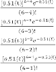
P 4 (t) = P 3 (t) = P 2 (t) =
P 1 (t) =
If we observe the bank for a period of 1 second, the probability of departing one customer in 0 to 1 seconds time interval is
0.306252744. If we observe the bank for 2 seconds, the probability of departing one customer in 0 to 2 seconds time interval is
0.367806838. If we observe the bank for 5 seconds the probability of departing one customer in 0 to 5 seconds time interval is
0.199108248. Up to 20 seconds the probabilities of departing n persons is calculated.
P 5 (1) = 0.306252744 P 4 (1) = 0.078094449
P 5 (2) = 0.367806838 P 4 (2) = 0.187581487
P 5 (4) = 0.26525857 P 4 (4) = 0.270563741 3
P 5 (5) = 0.19910824 P 4 (5) = 0.253863016
P 2 (1) = 0.00169269 P 1 (1) = 0.00017265
P 2 (2) = 0.01626331 P 1 (2) = 0.00331771
P 2 (3) = 0.04944062 P 1 (3) = 0.01512883
P 2 (4) = 0.093831505 P 1 (4) = 0.03828325
P 2 (5) = 0.137562022 P 1 (5) = 0.07015663
P 3 (1) = 0.013276056
P 3 (2) = 0.063777705
P 3 (3) = 0.129256529
P 3 (4) = 0.183983344
P 3 (5) = 0.215783565
Remaining values are tabulated.
Table-1 to Table-5 gives statistics of probabilities of arrivals of n
number of persons at time t.
1:
2:
IJSER © 2012
The research paper published by IJSER journal is about The effect of probabilities of departure with time in a bank 4
ISSN 2229-5518
ing n= 2, n = 3, n = 4, n = 5 and N = 6 respectively. By observing the graph, we would note that each curve peaks at a particular point and then they start to descend. After descending to a certain point
5:
Departure rate = 51 customers departing every 100 seconds. Scale: Time interval in seconds (0 to 20seconds)
P n (t) is 0 to 1
Departure rate = 0.51departures/second.
A graph is drawn between time and probability of n departures at time t. Time in seconds is taken on the horizontal line, P n (t) is taken on the vertical line. Curve-1 (c-1) is derived by taking N = 6 and n = 1 in the truncated Poisson probability distribution. As well remaining curves c-2, c-3, c-4, c-5 have been derived by tak-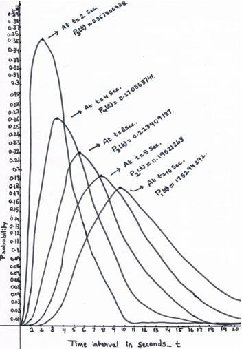
![]()
they run parallel to the time axis. We can observe that highest probability for curve-5 is at t = 2 seconds. This indicates probabili- ty of departure of one person from the bank from 0 to 2 seconds is high. Let ![]() denote the number of customers taken their service. Hear = 1. Curve-4 got highest point at t = 4 seconds. Third curve got highest point at time t = 6 seconds. Curve-2 got highest point at time t = 8 seconds. First curve got highest point at t = 10 seconds For the curve-1 at t = 10 seconds, the crest point P1 (10) =
denote the number of customers taken their service. Hear = 1. Curve-4 got highest point at t = 4 seconds. Third curve got highest point at time t = 6 seconds. Curve-2 got highest point at time t = 8 seconds. First curve got highest point at t = 10 seconds For the curve-1 at t = 10 seconds, the crest point P1 (10) =
0.175294292.
For the curve-2 at t = 8 seconds, the crest point P2 (8) =
0.195212635.
For the curve-3 at t = 6 seconds, the crest point P3 (6) =
0.223909187.
For the curve-4 at t = 4 seconds the crest point P4 (4) = 0.270563741.
For the curve-5 at t =2 seconds, the crest point P5 (2) = 0.367806838.
Developing appropriate formula for t at which we get highest
probability by use of crest points. Out of N = 6 customers, if 1 cus-
tomer had taken the service, then number of people remained in
the system is equal to 5. So we write n = 5 for which 1 customer
IJSER © 2012
The research paper published by IJSER journal is about The effect of probabilities of departure with time in a bank 5
ISSN 2229-5518
had taken service and 5 customers remained in the system. For n = 5 we have crest point at t = 2 seconds.
t = 2(1) seconds.
t = 2(number of customer who received the![]()
service) seconds.![]()
t = 2( ) seconds.
That is =1 (where ![]() is number of customers who received the service).
is number of customers who received the service).
For n = 4, we have crest point at t = 4 seconds.
t = 2(number of customers who![]()
received the service) seconds.
t = 2( ) seconds.
For n = 3, we have crest point at t = 6 seconds.
t = 2(3) seconds.
t = 2(number of customers who![]()
received the service) seconds.
t = 2( ) seconds.
For n = 2, we have crest point at t = 8 seconds.
t = 2(4) seconds
t = 2 (number of customers who![]()
received the service) seconds. .
t = 2( ) seconds.
For n = 1, we have crest point at t = 10 seconds.
t = 2(5) seconds.![]()
t = 2(number of customers who received the service) seconds. .
t = 2( ) seconds.
The above calculations can be generalized and is indicated by the
following formula.
For the departures in a queueing system which follow truncated
Poisson probability distribution, t = 2(N-n) seconds is the time
where we get maximum probability for the curves c-1, c-2, c-3 etc
and N, n are positive integers.
This paper studies the Queueing theory and by the use of queuing
theory analysis of probability curves of pure death model. From
the work surveyed above we have found departure rate at the bank is 0.51 departures per second. We Considered the Random
variable as “Number of departures during the time interval 0 to t” which follows truncated Poisson probability distribution. We calculated probabilities of departures of n = 1, 2, 3, 4, 5 persons during time interval 0 to t. A graph was drawn between the time and probabilities of n departures where n = 1, 2, 3, 4, 5 from which curves c-1, c-2, c-3, c-4 and c-5 were obtained. By observing the graph, we would note that each curve peaks at particular point and then they starts to descend. That is each curve had peak point at particular time. From the above calculations we developed an equation to find this particular time t where curve attain its crest point. The equation is (Time) t = 2(N-n) seconds where N is the number of customers allowed at initial time 0 seconds, n is the number of customers remained in the system after taking N-n people service. This equation assists us in deriving time where curve takes crest point.
We observe that if n increases, P n (t) increases. That is n ∞ P n (t).
If t increases P n (t) decreases.
[1] Fundamentals of Queueing theory by James M Thomson, Do- nald Gross; Wiley series.
[2] Operations research by Hamdy Taha. [3] Operations research by S.D Sharma.
[4] Queueing theory and its applications; A personal view by Ja- nus Sztrik. Proceedings of the 8th International conference on Ap- plied Informatics, Eger, Hungary, Jan 27-30, 2010, Vol.1, PP.9-30.
[5] Case study for Restaurant Queueing model by Mathias, Erwin.
2011 International conference on management and Artificial
Intelligence. IPDER Vol.6 (2011) © (2011) IACSIT Press, Bali, In-
donesia.
[6] A survey of Queueing theory Applications in Healthcare by
Samue Fomundam, Jeffrey Herrmann. ISR Technical Report 2007-
24.
[7] An application of Queueing theory to the relationship between
Insulin Level and Number of Insulin Receptors by Cagin Kande-
min-Cavas and Levent Cavas.
Turkish Journal of Bio Chemistry-2007; 32(1); 32-38
[8] The Queueing theory of the Erlang Distributed Inter arrival
and Service time by Noln Plumchitchom and Nick T Thomopou-
los.
Journal of Research in Engineering and technology; Vol-3, No-4,
October-December 2006.
[9] Queueing theory in Call centers by Ger Kook and Avishai-
Mandelbaums.
The Netherlands Industrial engineering and Management, Tech-
nion, Haifa, 32000, Israel, October-2001.![]()
That is t ∞ .
IJSER © 2012
Internatio nal Jo urnal of Scientific & Engineering Research Volume 3, Issue 7, July-2012 6
ISSN 222S-5518
IJSER lb)2012
htt p://www .'lser. ora