International Journal of Scientific & Engineering Research Volume 4, Issue 2, February-2013 1
ISSN 2229-5518
Nitin Bhardwaj, Ashok Kumar, Jasdev Bhatti
—————————— ——————————
ABSTRACT: Generally consider that failure and repair times of a unit are continuous distribution. But, in practice the situation exist when the failure and repair of a unit occur at discrete random epoch so that the life time and repair time of a unit follow discrete distribution, like geometric, negative binomial, Poisson etc. actually, discrete failure data arise in several common situations for example in a photo copy machine the bulb is lightened every time when a copy is taken. Thus, the life time of the bulb is discrete random variable.
Keeping the above concept of discrete time modelling we in the present paper analyse a two, identical unit is via partial system with imperfect switching. Initially one unit is operative and othet is stand by, we consider two types of failures, partial failure and total failure. Failure and time of the unit are considered as Geometric distribution. Various measures of system effectiveness are also obtained.
Keywords: Geometric distribution, redundant system, discrete random variable.
In some situation, discrete failure time distributions are appropriate to model “lifetimes”. For example, discrete distribution is appropriate when a piece of equipment operates in cycles and the number of cycles prior to failure is observed.
Discrete failure data arise in several common situations, for example: a) A device is monitored only once per time period (e.g, an hour, a day), and the observation is the number of time periods successfully completed prior to failure of the device. b) A piece of equipment operates in cycles and the experimenter observes the number of cycles successfully completed prior to failure.
In situations where the observed data values are very large (in thousands of cycles, etc.) a continuous distribution is
an adequate model for the discrete random variable. However
when the observed values are small, continuous distribution might not adequately describe a discrete random variable.
The purpose of this paper is to incorporate the concept of discrete distribution. Generally consider that failure and repair times of a unit continuous distribution of time to failure and time to repair of a unit. However, in practice the situation exists when the failure and repair of a unit occur at discrete random epochs so that the life time and repair time of a unit follows discrete distribution like geometric, negative binomial, poission etc.
Some examples of discrete life times are as follows:
“In a photo copy machine the bulb is lightened every time when a copy is taken. Thus, the life time of the bulb is a discrete random variable”.
“In an on /off switching device, the life time of the switch is a
discrete random variable”.
IJSER © 2013 http://www.ijser.org
International Journal of Scientific & Engineering Research Volume 4, Issue 2, February-2013 2
ISSN 2229-5518
“In a refrigerator, the bulb is lightened whenever the door of the refrigerator is opened. Thus, the life time of the bulb is the discrete random variable”.
Thus, we see that many practical situations of importance are represented with the help of discrete life time models. Similarly, the repair time may be considered as discrete random variable as dividing the whole time interval into various small parts of time. Discrete time models are considered by several researchers including Padgett and Spurrier [1985], Salvia and Bollinger [1982], J.F.Lawless [1982], Kalbfleish and Prentice [1980] etc.
This model consists of two-unit, the main unit and the standby unit. It is assume that main unit can work in normal mode i.e. with full efficiency. The single repairman facility is available with the system to repair the failed unit and repair the switch. First priority of the repairman is repair to the failed switch. For both the units, the distribution of time to failure and repair is taken as geometric distribution and repair time distribution of the switch is also geometric distribution. Using regenerative point technique, the following reliability characteristics of interest have been obtained.
(i) Distribution of time to system failure and its mean.
(ii) Pointwise and steady state availability of the system
(iii) Expected busy period of repairman in [0, t] and in steady state.
(iv) Expected profit incurred in [0, t] and in steady state.
Few characteristics such as MTSF, system availability and profit in steady state have also been studied through graphs.
System is analysed under the following assumptions.
(i) A cold standby system consists of two-identical unit one is operative and other is standby. Each unit has two-modes: normal (N), and total failure (F). The standby-unit cannot fail.
(ii) Failure is self announcing state operating.
(iii) Switching is imperfect in the transition from standby state to operating state.
(iv) A single repairman is available to repair a failed unit and switch.
(v) The failure and repair time distribution of the unit are independent having geometric distribution with parameter p and r2.
(vi) The repair time distribution of the switch is independent having geometric distribution with parameter r1.
(vii) The failure times of the unit are taken as independent random variable.
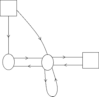
2.1 Notations and States of the Systems N0 : unit in normal mode and operative Ns : unit in normal mode and standby
Fr|Fwr : unit in failure mode and under repair| waiting for repair
Sr : Switch failed and under repair SFNs : Switch failed unit in standby state Up State Down State
S0 (N0, Ns), S1 (Fr, N0) S2 (Fr, Fwr), S3 (Fwr, SFNs)
IJSER © 2013 http://www.ijser.org
International Journal of Scientific & Engineering Research Volume 4, Issue 2, February-2013 3
ISSN 2229-5518
a : The probability that switch is perfect
Pij =
lim Qij
t
b : The probability that switch is imperfect
S3
Fwr
SFNs
Sr
P01 + P03 = 1 P10 + P11 + P12 = 1 P21 = P31 = 1
Let Ti be the sojourn time in state Si(i = 0, 1) then mean sojourn time in state Si is given by
so that
1
bp 1
![]()
S 0 =
i =
t 0
P(Ti > t)
1
![]()
1 =
S0 a
N0 p
S1 s2p
Fr
Fr
1 q
1
1 s2 q
1
Ns r2q r2
Fwr
2 =
![]()
1 s2
3 =
![]()
1 s1
(1.8 -1.11)
r2p
Defining mij as the mean sojourn time of the system in state Si
when the system is transit into state Sj i.e.![]()
Operative state
mij =
t 0
t qij(t)
![]() Failed state
Failed state
m01 + m02 = 0 m10 + m11 + m12 = qs2 1
m31 = s1 3 m21 = s2 2
To obtain the distribution of the time to system failure we
Q01(t) = ap
1 q( t 1)
![]()
1 q
Q03(t) = bp
1 q( t 1)
![]()
1 q
regard the failed states as absorbing states. By using
probabilistic argument, the following recursive relation for
Q01(t) = r2q![]()
[1 (qs2
) t 1 ]
Q11(t) = r2p![]()
[1 (qs2 ) t 1 ]
Ri(t) :
1 qs2
1 qs2
R (t) = z (t) + q
(t1) R (t1)
0 0 01 1
[1 (qs
) t 1 ]
[1 s (t 1) ]
R1(t) = z1(t) + q10(t1) R0(t1) + q11(t1) R1(t1) (1.12 – 1.13)
Q12(t) = ps2 2
1 qs2
[1 s (t 1) ]
Q21(t) = r2 2
1 s2
Taking geometric transform on both sides
We get
Q31(t) = r1 1
1 s1
(1.1 – 1.7)
R * (h)
![]()
N1 (h)
D1 (h)
The steady state transition probabilities from state Si to Sj can
be obtained from
where,
IJSER © 2013 http://www.ijser.org
International Journal of Scientific & Engineering Research Volume 4, Issue 2, February-2013 4
ISSN 2229-5518
N1(h) =![]()
Z* (h)
hq*
![]()
(h)
N2(h) =
Z* (h)
![]()
1 hq* (h)
Z* (h)
hq*
(h)
0 hq*
![]()
(h)
N1(h) = Z* (h)[1 hq* (h)] hZ* (h)q*
(h)
Z* (h)
1 hq* (h)
hq*
(h) 0
0 11
and
1 01 0
0
![]()
*
hq*
hq*
(h) 1 0 (h) 0 1
![]()
D1(h) = 1
hq 01(h)
N2(h) = Z*(h)(1hq* (h))h2q* (h)q* (h)Z*(h) hq* (h)Z*(h)
hq* (h)
1 hq* (h)
0 11
12 21 0
01 1
+ h2 q* (h)q* (h)Z* (h)
D1(h) = 1h q* (h) h 2q*
(h)q*
(h)
31 03 1
Then MTSF = lim
11 01 10
![]()
N1 (h) 1
D2(h) =![]()
1
hq* (h)
hq* (h)
1 hq* (h)
0
hq* (h)
![]()
hq* (h)
0
MTSF =
h 1 D1 (h)
![]()
N1
0
0
(1.14)
hq* (h) 1 0
hq* (h) 0 1
D1 D2(h)=1h q* (h) h 2q* (h)q* (h) h2q* (h)q* (h) h3q* (h)q* (h)q* (h)
where
11
where,
12 21
01 10
03 10 31
N1 = 0(1 P11) + 1P01 + P11 + P01 P10 1
D1 = 1P11 P01 P10
Let Ai(t) be the probability that the system is up at epoch t when it is initially started from regenerative state Si by simple
Z0(t) = qt Z1(t) = (sq)t
The steady state availability of the system is given by
A0 = lim A0 (t)
t
hence, by applying ‘L’ Hospital Rule we get
probabilistic arguments the following recurrence relations are obtained.
A0(t) = Z0(t) + q01(t1) A1(t1) + q03(t1) A3(t1)
A1(t) = Z1(t) + q10(t1) A0(t1) + q11(t1) A1(t1) + q12(t1)
A2(t1)![]()
A0 = N 2 (1) D2 (1)
N2(1) = 0(1P11 P12) + 1(P01 + P03)
D2(1) = {qs2 1 + 0 P10 + P03 P10 s13 + P12 s2 2}
(1.19)
A2(t) = q21(t1) A1(t1)
A3(t) = q31(t1) A1(t1) (1.15 – 1.18) By taking geometric transformation on both sides and solving the equations.
N2 (h)
![]()
A0*(h) =
D2 (h)
By probabilistic argument, we have the following recursive
relation for Bi
B0(t) = q01(t1) B1(t1) +q03(t1) B3(t1)
B1(t)=Z1(t) +q10(t1)B0(t1)+q11(t1) B1(t1) + q12(t1)B2(t1) B2(t) = Z2(t) + q21(t1) B1(t1)
B3(t) = Z3(t) + q31(t1) B1(t1) (1.20-1.23)
By taking geometric transform on both sides and solving the
where
equations.
IJSER © 2013 http://www.ijser.org
International Journal of Scientific & Engineering Research Volume 4, Issue 2, February-2013 5
ISSN 2229-5518
![]()
where
N3(h) =
B0*(h) =
0
Z* (h) Z* (h) Z* (h)
![]()
N3 (h) D 2 (h)
hq* (h)
1 hq* (h)
hq* (h)
hq* (h)
0
hq* (h)
1
0
hq*
0
0
1
(h)
Using the above equation and equation (1.14), (1.19), (1.24) and (1.25) we can have the expression for MTSF, availability etc. for this particular case.
On the basis of the numerical values taken as:
The values of various measures of system effectiveness are obtained as:![]()
N3(h)=h q* (h)Z* (h) hq* (h)Z* (h) h 2q* (h)q* (h)Z* (h) hq* (h)
01 1
12 2
03 31 1 03
(1 hq* (h))Z* (h) h 3q* (h)q* (h)q* (h)Z* (h) h3
11 3
12 03 31 2
q* (h) q* (h) q* (h)Z* (h)
12 21
03 3
For the graphical interpretation, the mentioned particular case
and D2(h) is the same as in availability analysis
B0 = lim B0 (t)
t
Hence, by applying ‘L’ Hospital Rule, we get![]()
B0 = N3 (1) D2 (1)
where
N3(1) = 1 + 2P12(1 + P03) + 3 P03(1P11 P12)
and D2(1) is the same as in availability analysis
The expected total profit in steady-state is
(1.24)
is considered.
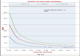
(p). It is clear from the graph that the MTSF get decrease with increase in the value of failure rate.
(r2). It is clear from the graph that the MTSF gets increase with increase in the value of repair rate.
where
P = C0 A0 C1B0 (1.25)
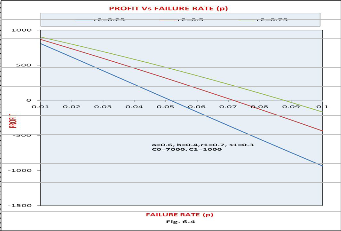
rate (p) for different values of repair rate (r2). The profit
decreases with the increase in the value of failure rate (p) and
C0 be the per unit up time revenue by the system and
C1 be the per unit down time expenditure on the system.
is higher for higher values of repair rate (r2). Following can also be observed from the graph:
P01 =
ap
![]()
1 q
r q
, P03 =
bp
![]()
1 q
r p
(i) For r2 = 0.25, P > or = or < 0 according as p < or =
or > 0.0518. So, the system is profitable only if
P10 = 2 , P11 = 2 ,
failure rate is less than 0.0518.
1 qs2
ps2
P12 =
1 qs2
1 qs2
P21 = 1, P31 = 1
(ii) For r2 = 0.5, P > or = or < 0 according as p < or = or
> 0.0725. So, the system is profitable only if failure rate is less than 0.0725.
IJSER © 2013 http://www.ijser.org
International Journal of Scientific & Engineering Research Volume 4, Issue 2, February-2013 6
ISSN 2229-5518
(iii) For r2 = 0.75, P > or = or < 0 according as p < or = or > 0.0878. Thus the system is not profitable when > 0.0878.
So, the companies using such systems can be suggested to purchase only those system which do not have failure rates greater than those discussed in points (i) to (iii)
above in this particular case.
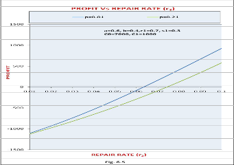
Fig. 1.5 shows the pattern of the profit with respect to repair rate (r2) for different values of failure rate (p). The profit
increases with the increase in the value of repair rate (r2) and is lower for higher values of failure rate (p). Following can also be observed from the graph:
(i) For p = 0.01, P > or = or < 0 according as r2 > or = or < 0.06324. So, the system is profitable only if repair rate is greater than 0. 06234.
(ii) For p = 0.21, P > or = or < 0 according as r2 > or = or < 0.07374. Thus the system is not profitable when ≤ 0.07374.
So, the companies using such systems can be suggested to
purchase only those systems which do not have repair rates greater than those discussed in points (i) to (ii) above in this particular case.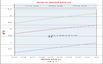
IJSER © 2013 http://www.ijser.org
International Journal of Scientific & Engineering Research Volume 4, Issue 2, February-2013 7
ISSN 2229-5518
[1] Bhatti J, Chitkara A, Bhaedwaj N (2011), “ Profit analysis of two unit cold stanby system with two types of failure under inspection policy and discrete distribution”, IJSER, Volume 2, Issue 12, Dec. – 2011.
[2] Agarwal S.C, Sahani M, Bansal S (2010) “Reliability
characteristic of cold-standby redundant syatem”, May 2010 3(2),
IJRRAS.
[3] Bhardwaj N (2009) “Analysis of two unit redundant system with imperfect switching and connection time”, International transactions in mathematical sciences and Computer,July-Dec.
2009,Vol. 2, No. 2, pp. 195-202.
[4] Bhardwaj N, Kumar A, Kumar S (2008) “Stochastic analysis of a single unit redundant system with two kinds of failure and repairs”, Reflections des. ERA-JMS, Vol. 3 Issue 2 (2008), 115-134
[5] Gupta R, Varshney G (2007) “A two identical unit parallel
syatem with Geometric failure and repair time distributions”, J. of comb. Info. & System Sciences, Vol. 32, No.1-4, pp 127-136 (2007)
[6] Taneja G, Tyagi V K, Bhardwaj P (2004) “Profit analysis of a
single unit programmable logic controller (PLC), Pure Appl.
Math. Sci., vol. LX 1-2, September 2004.