International Journal of Scientific & Engineering Research Volume 4, Issue 2, February-2013

ISSN 2229-5518

Super-Resolution Mosaicing of Unmanned Aircraft

System (UAS) Surveillance Video Frames

Debabrata Ghosh, Naima Kaabouch, and William Semke

Abstract- Unmanned Aircraft Systems have been used in many military and civil applications, particularly surveillance. However, video frames are often blurry, noisy, and exhibit insufficient spatial resolution. This project aims to develop a vision-based algorithm to improve the quality of UAS video frames. This algorithm will be able to generate high resolution mosaic output through a combination of image mosaicing and super-resolution (SR) reconstruction techniques. The mosaicing algorithm is based on the Scale Invariant Feature Transform, Best Bins First, Random Sample Consensus, reprojection, and stitching algorithms. A regularized spatial domain-based SR algorithm is used to super resolve a mosaic input. The performance of the proposed system is evaluated using three metrics: Mean Square Error, Peak Signal-to-Noise Ratio, and Singular Value Decomposition-based measure. Evaluation has been performed using 36 test sequences from three categories: images of 2D surfaces, images of outdoor 3D scenes, and airborne images from an Unmanned Aerial Vehicle. Exhaustive testing has shown that the proposed SR mosaicing algorithm is effective in UAS applications because of its relative computational simplicity and robustness.

Index terms- SIFT, Mean Square Error, Peak Signal-to-Noise Ratio, Singular Value Decomposition, regularization parameter, Huber prior, Laplacian prior.

—————————— · ——————————

1 INTRODUCTION

IGITAL images are often limited in quality because of the imperfections of the image-capturing devices (e.g., limited sensor density, finite shutter speed, finite shutter

time, and sensor noise) and instability of the observed scene (e.g., object motion and media turbulence). However, UAS applications require higher quality images to facilitate better content visualization and scene recognition. Since constructing optical components to capture such high resolution images is prohibitively expensive and not practical in real applications such as UAS surveillance operations, a more feasible solution is to use signal processing to post-process the acquired low quality images [1]. Undoing the effect of blur and noise from an image does not address the low spatial resolution problem. Image interpolation, on the other hand, increases the size of a single image. However, the quality of an image magnified from an aliased low resolution image is inherently of poor quality. If interpolation along with restoration can be performed on a sequence of images, depicting the same underlying scene, additional information from multiple images can be fused to construct a super resolution image.

————————————————

• Debabrata Ghosh is currently pursuing a PhD degree program in the department of Electrical Engineering at the University of North Dakota, Grand Forks, USA, 58203. E-mail: debabrata.ghosh@my.und.edu

• Naima Kaabouch is an Associate Professor in the department of Electrical Engineering at the University of North Dakota, Grand Forks, USA, 58203. E-mail: naima.kaabouch@engr.und.edu

• William Semke is an Associate Professor in the department of Mechanical

Engineering at the University of North Dakota, Grand Forks, USA, 58203.

E-mail: william.semke@engr.und.edu
The combination of image mosaicing and super-resolution reconstruction, i.e. super-resolution mosaicing, is a powerful means of representing all of the information of multiple overlapping images to obtain a high resolution panoramic view of a scene. The stability of a super-resolution mosaicing method requires that multiple images are correlated solely by planar homography. Two important situations where consecutive images are exactly correlated by planar homography are: images of a plane produced by a camera which purely rotates about its optical center and images produced by a camera zooming in or out of the scene. These two situations guarantee that images do not show parallax effect, i.e. the scene is approximately planar [2]. Under these circumstances, the underlying scene can be reconstructed with higher resolution from the correlated frames.
Several mosaicing algorithms and super resolution reconstruction algorithms have been proposed over the last decades [3]-[9]. Some of these algorithms include super resolution image reconstruction using the ICM algorithm proposed by Martins [10], self-adaptive blind super-resolution image reconstruction proposed by Bai [11], super resolution image reconstruction based on MWSVR estimation proposed by Cheng [12], and super resolution image reconstruction based on the minimal surface constraint on the manifold proposed by Yuan [13]. However, very little work has been done for super resolution mosaicing, which encompasses both a SR algorithm and a mosaicing algorithm at the same time. Furthermore, as algorithms have become more accurate in recent years, the necessity for quantitative evaluation has become more and more necessary.
Tian et al. [14] reconstructed SR images from several LR images generated from high resolution (HR) frames. They used a ground truth and three different metrics to evaluate the performance of the SR technique objectively. However, availability of the ground truth is unlikely in most real

International Journal of Scientific & Engineering Research Volume 4, Issue 2, February-2013

ISSN 2229-5518

applications and, furthermore the performance metrics lack simplicity because they require computing SIFT feature points and segments from images. Kim et al. [15] used ground truth
Using deterministic regularization, the constrained least square (CLS) can be formulated as:

2 2

along with four different performance metrics for quantitative
evaluation. However, in spite of their complicated algorithms,
human visual system-based objective measures (eg. structural
similarity, color difference equations) do not appear to be
superior to simple pixel-based measures like mean square
error and peak signal-to-noise ratio. Additionally, the

x� = yk - DBk Wk R[x]k 2 + A Lx 2

k=l

(3)

dynamic range of structural similarity is too small to compare quantitatively the performance of SR mosaicing algorithms.
This paper describes a SIFT based mosaicing algorithm along with a regularized spatial domain based SR algorithm to perform SR mosaicing. To assess the effectiveness of the proposed algorithm three computationally very simple metrics are used.

2 BACKGROUND

A real scene gets warped by the camera lens because of the relative motion between the scene and the camera. Thus the inputs to the camera are multiple frames of a real scene connected by local or global shifts. In addition, frames are often degraded by blurring effects and noises. Finally, the camera sensor discretizes (downsamples) the frames which result in digitized, blurry, and noisy frames. Based on the aforementioned image formation model, super resolution mosaicing is an inverse problem i.e. achieving the SR mosaic from the observed LR frames. A single observation makes the inverse problem heavily underdetermined, resulting in an unstable solution [16]. Thus, if we assume K numbers of LR

x� = arg minx yk - DBk Wk R[x]k 2

k=l

+ A p(g, a) (4)

gEG(x)

Equation (3) uses the Laplacian prior, whereas the equation (4) uses the Huber prior. The advantage of the Huber prior is that it penalizes the edges less severely than the Laplacian prior. A is the regularization parameter, L is the Laplacian
operator, p(g, a) is the Huber function. G(x) is the set of
gradient estimates over the cliques [19]. a represents a
gradient which changes the penalty from non-linear to linear
as follows:

x2 if x ::; a p x a

2a|x| - a2 , otherwise

Gradient descent algorithm can be used to minimize the
cost functional in (3) or (4). According to the analysis in [15]
the iterative update for x� can be expressed as

T T T n K

frames are available, the kth LR image can be represented as:

x�(n+l) = x�n + /](n) {RT [Wk Bk D

(yk - DBk Wk R[x�

]k )]k=l

yk = DBk Wk R[x]k + nk for 1 ::; k ::; K (1)

Where x is the SR mosaic; D, Bk , Wk and nk are decimation

- An LT Lx�n } (6)

T BT DT (y

- DB W R[x�n ] )]K

operator, blur matrix, warp operator and the additive noise,

x�(n+l) = x�n + /](n) {RT [Wk k k

k k k

k=l

respectively. The reconstruction of the kth warped SR image
from x is represented by R[. ]k [17].

- An GT pt(Gx�n , a)} (7)

It is obvious that finding an estimate of a SR mosaic is not

Where �(n) is the step size of the nth iteration, D

is the
solely based on the availability of captured LR frames. Rather, it depends on several other specifications, such as the blurring process and the noise. If the blur is assumed to be linear and spatially invariant, it could be modeled by convolving the image with a low-pass filter. Noise is assumed to be additive white Gaussian noise in the above image acquisition model. From equation (1), the maximum likelihood estimate of the SR
interpolation operator, W T is the forward warping operator
(assuming W to be the backward warping operator), BT
represents convolution with a PSF kernel which is flipped to
the PSF kernel used to model the B operator.
According to [20], regularization parameter An can be
expressed as follows.

mosaic x� is

An =

k=l

yk - DBk Wk R[x�n ]k 2

Lx�n 2

for equation (6) (8)

x� = arg minx yk - DBk Wk R[x]k 2 (2)

k=l

LK yk - DBk Wk R[x� n ]k 2

Where . 2 is the 2-norm. SR mosaicing is an ill-posed
problem because of an insufficient number of LR frames and
ill-conditioned blur operators [18].
In order to make the SR mosaicing process a well-posed problem, prior information is added in the solution space.

An =

k=l

p(Gx� n , a)

for equation (7) (9)

International Journal of Scientific & Engineering Research Volume 4, Issue 2, February-2013

ISSN 2229-5518

3 APPROACH

The proposed system uses a combination of a mosaicing algorithm and a super resolution algorithm. The mosaicing system is based on the Scale Invariant Feature Transform (SIFT), Best Bins First (BBF), Random Sample Consensus (RANSAC), reprojection and stitching algorithms. The SR system, on the other hand, is based on a deterministic regularization algorithm, which uses gradient descent optimization in order to minimize the cost functional in (3) or (4) as discussed in the previous section.
Fig. 1 shows the flowchart of the mosaicing algorithm. This algorithm reads the input frames and applies SIFT algorithm to extract feature points from these frames. SIFT uses five steps: scale-space construction, scale-space extrema detection, keypoint localization, orientation assignment, and defining keypoint descriptors. Initially, a Gaussian filter with variable scale is employed to construct the scale-space. Once it constructed, the difference of Gaussian scale-space is computed and extrema are detected by comparing a pixel to its 26 neighbors at the current and adjacent scales. In order to discard the undesirable low contrast and roughly localized key points keypoint localization is used. For each key point one or more orientation assignments are determined using the local image gradient directions. These orientation values are then accumulated into an orientation histogram that summarizes the contents over 4x4-pixel neighborhoods with 8 bins each [21]. Finally, a 128 dimension descriptor vector is assigned to each key point.
SIFT feature points extracted from a sequence of images are stored into databases. BBF algorithm (a modified version of the k-d tree) is then used to estimate the initial matching points between image pairs. This is achieved by finding the nearest neighbor of a keypoint in the first image from a database of keypoints for the second image. Keypoint with the minimum Euclidean distance for a 128 dimension descriptor vector is regarded as nearest neighbor.
RANSAC algorithm uses those initial matching points and
removes the outliers to estimate an optimum homography
matrix based on homography constraints (geometric distance
error, maximum number of inliers, etc.). The homography
matrix is a 3x3 matrix that takes into account several image
transformation parameters. To compute this matrix, one of the
input frames is assigned as the reference frame and the current
homography matrix is multiplied with all the previous
homograph matrices until the reference frame is reached.
Using the homography metrics, images are warped into a
common coordinate frame.
Finally, stitching is employed to obtain the final mosaicing output. To achieve the stitching, each pixel in every frame of the scene is checked for whether it belongs to the warped second frame or not. If it belongs, then that pixel is assigned
the value of the corresponding pixel from the second frame. Otherwise, it is assigned the value of the corresponding pixel from the first frame.
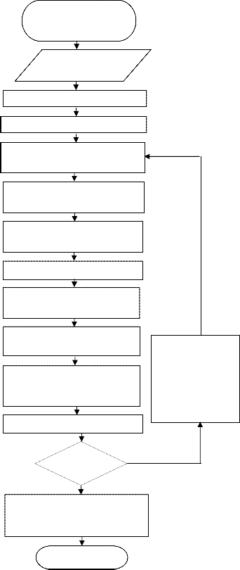
Fig. 2 shows the flowchart of the SR mosaicing algorithm. The system takes LR frames and the maximum number of iterations as inputs to the algorithm. After the input LR frames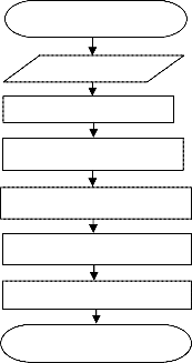

are interpolated, a mosaic (say the initial mosaic) is computed out of those interpolated LR frames. Inverse mosaicing is used to reconstruct the LR frames from the mosaic. This inverse mosaicing makes use of inverse warping and downsampling to find the reconstructed LR frames. Inverse warping utilizes the same homography metrics that were used in warping the LR frames to the reference frame while making the initial mosaic. Those reconstructed frames are then subtracted from

Start

Input frames SIFT feature extraction SIFT matching using BBF

RANSAC for homography Reprojection of frames Stitching multiple frames End of mosaicing algorithm

Fig. 1. Flowchart of the mosaicing system

the original LR frames to find the difference images. The difference images are similarly interpolated and an error mosaic is computed using all of these images. This error mosaic is added to a regularization term and subsequently used to update the initial mosaic. This process is repeated iteratively to minimize the cost functional in Equation (3) or Equation (4) until the maximum number of iterations has been reached.
Conceptually, the regularization parameter should be chosen such that it gets smaller with the progress of the iterative process as we would be moving toward a better solution. The numerators of the regularization parameters in both equations (8) and (9) are the error energy, which is the difference between the original LR frames and the reconstructed LR frames. This error energy becomes smaller as the iteration proceeds. The denominators of both equations (8) and (9), on the other hand, increase as the iterative process advances. This is because this iterative algorithm tries to
restore the high frequency components in x� n. Thus both the
regularization parameters in equations (8) and (9) decrease
with the iteration. � in the flowchart expresses the step size of
the algorithm for an iteration. To make the step size adaptive,
it is allowed to change at every iteration based on the term:

International Journal of Scientific & Engineering Research Volume 4, Issue 2, February-2013

ISSN 2229-5518

mosaic of interpolated difference images - regularization term. Fig. 3 illustrates the schematic of the algorithm.
To make the evaluation process as controllable as possible, synthetic image frames are created by using several wide- angle reference color images and then creating overlapping input data. The wide-angle reference images act as real-world sceneries. The most common camera-related transformation (translation) is applied to the input data. Data frames are created in such a way that the consecutive frames have at least a 50% overlapping region., which is regarded as one of the requirements of the SIFT algorithm. The process of generating the sequence of input data frames simulates the real situation of photographing multiple shots that cover different areas of a scene. The generated frame sequence is added to different synthetic blurs within acceptable margins. This sequence of frames is then fed to the SR mosaicing algorithm and the super resolved mosaic image is obtained. The SR mosaicing algorithm requires the size of the panorama frame as well as the offset in both x and y directions. These offsets are required to make sure a complete view of the mosaic output is obtained.
Finally, the initial mosaic without SR and the output super resolved mosaic are compared to evaluate the performance of the SR mosaicing algorithm, we used three metrics: mean square error, peak signal-to-noise ratio, and singular value decomposition-based measure. These metrics are calculated and compared for the initial mosaic without SR and the output super resolved mosaic.

1) Mean Square Error

Beginning of the SR

algorithm

LR input frames and max_iter

Interpolation of LR frames

Iter=1

Mosaicing of interpolated LR images

Reconstruction of LR frames via inverse mosaicing

Difference image of the original and reconstructed LR image

Interpolation of difference images

Mosaicing of interpolated difference images

The mean square error (MSE) is used as a measurement of the effectiveness of the SR mosaicing algorithms. MSE represents the mean of the squared differences for every pixel.

Li Lj(I(i,j)-O(i,j

Mosaic of interpolated difference images- Regularization term

� (Mosaic of interpolated difference

� (Mosaic of interpolated difference images-

MSE =

(10)

images- Regularization term)+ Mosaic of interpolated LR images

Regularization term)+

Mosaic of interpolated LR

Where, I(i,j) and O(i,j) are the (i,j) th pixel values in the
initial mosaic and the final SR mosaic respectively. N is the
total number of pixels in each image.
The lower the similarity between two images, the higher
the MSE between them.

2) Peak Signal- to-Noise Ratio

Iter=Iter+1

Iter<max_iter

Yes

images

The peak signal to noise ratio (PSNR) is used as a measurement of the difference between two images. PSNR of corresponding pixel values is defined as

� (Mosaic of interpolated difference images- Regularization term)+ Mosaic

of interpolated LR images

PSNR = 10 log10 (max (I(i,j),O(i,j))) MSE

(11)

End

Where, MSE is the mean square error. PSNR is expressed in decibels (dB) and a lower value corresponds to a higher difference between two images.

Fig. 2. Flowchart of the SR mosaicing system

International Journal of Scientific & Engineering Research Volume 4, Issue 2, February-2013

ISSN 2229-5518

3) Singular Value Decomposition-based measure

Singular value decomposition (SVD)-based measure is used to express the amount of distortion in terms of dissimilarity between two images. Any real matrix M of size mxn can be
decomposed into a product of 3 matrices M = USVT, where U
and V are orthogonal matrices of sizes mxm and nxn,
respectively. S is an mxn diagonal matrix with the singular
values of M as its diagonal entries. The columns of U are left
singular vectors of M, whereas the columns of V are called
right singular vectors of M [22]. The left singular vectors of M
are eigenvectors of MMT and the right singular vectors of M are eigenvectors of MTM. The non-zero singular values of M are the square roots of the non-zero eigenvalues of both MMT and MTM. Considering each image as a real matrix, a global
SVD can be computed. Subsequently, the distance between the two sets of singular values corresponding to the mosaic with SR image and mosaic without SR image can also be measured as below.
the SVD-based measure corresponds to a higher degree of difference between two images.
As super resolution inherently means increasing the resolution of an image by restoring the lost frequency components, thus higher values of MSE or SVD-based measure between the initial mosaic and the final SR mosaic indicate better performance of the SR mosaicing algorithm compared to the lower values for those metrics. Similarly, a lower PSNR values between the mosaic without SR and mosaic with SR images correspond to improved performance of the SR algorithm.

4 RESULTS AND DISCUSSION

A total of 36 data sets (10 sets in each of the three categories) of 5 frames each have been used to evaluate the efficiency of the SR mosaicing algorithm. These data sets fall into three categories: 2D surface images, real 3D scene images, and airborne images from an Unmanned Aerial Vehicle (UAV)

N obtained during a 2011 University of North Dakota (UND)

2 flight test. These frames were downsampled and added to

D = sqrt - (12)

Where Si is the singular values of the initial mosaic image,
S�i is the singular values of the final SR mosaic image, and N is
the total number of pixels in each image. A higher value for
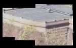
blur using a circular averaging filter of radii 1 and 2 to generate input sequence for the SR mosaicing algorithm. Fig.
4, 5, and 6 show examples of results for each category of the
SR mosaicing algorithm. The maximum number of iterations
was chosen as 7 for all the three categories. This is the stopping criterion for the iterative procedure.

Fig. 3. Schematic of the SR system

International Journal of Scientific & Engineering Research Volume 4, Issue 2, February-2013

ISSN 2229-5518

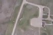
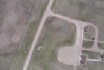
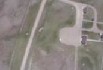
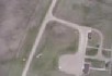
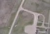
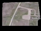
However, the error between two successive steps of iterations can also be used as a stopping criterion. Fig. 4 shows an example of a 2D scene consisting of 5 frames (Fig. 4 a, b, c, d, and e) and their corresponding SR mosaicing output (Fig. 4 f). Fig. 5 shows an example of a 3D scene consisting of 5 frames (Fig. 5 a, b, c, d, and e) and their corresponding SR mosaicing output (Fig. 5 f). Fig. 6 shows an example of a UAV scene consisting of 5 frames (Fig. 6 a, b, c, d, and e) and their corresponding SR mosaicing output (Fig. 6 f). The input frames are blurry as we can see from the figures. It can be clearly visualized that the SR mosaicing algorithm has successfully generated higher resolution mosaicing output from those input frames. Fig. 7 and Fig. 8 show a subjective comparison of the mosaic without SR and mosaic with SR algorithm. Fig. 7 and Fig. 8 show a subjective comparison of the mosaic without SR and mosaic with SR algorithm.

(a) (b) (c)

(d) (e)

(a)

(b)

(d) (e)

(f)

(c)

(f)

Fig. 5. Example of results corresponding to real 3-D data sequence of frames and their corresponding SR mosaicing output:

(a),(b),(c),(d), and (e) Input image frames

(f) Corresponding SR mosaicing output

(a) (b) (c)

Fig. 4. Example of results corresponding to 2-D data sequence of frames and their corresponding SR mosaicing output:

(a),(b),(c),(d), and (e) Input image frames

(f) Corresponding SR mosaicing output

(d) (e)

(f)

Fig. 6. Example of results corresponding to real UAV data sequence of frames and their corresponding SR mosaicing output:

(a),(b),(c),(d), and (e) Input image frames

(f) Corresponding SR mosaicing output

International Journal of Scientific & Engineering Research Volume 4, Issue 2, February-2013

ISSN 2229-5518

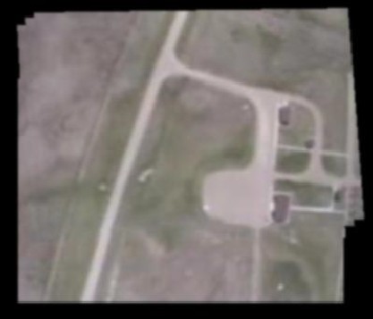
Fig. 7. Mosaic without SR using one of the UAV data sequences

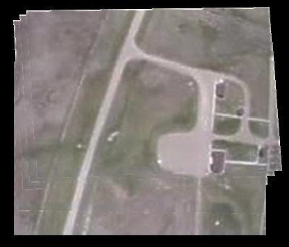
Fig. 8. Corresponding mosaic with SR

Higher values of MSE and SVD based measure indicates that the SR mosaicing recovers more high frequency components and hence it gives a smaller PSNR value. When there is no added blur to the input sequence, the MSE and
SVD based values between the mosaic without SR and mosaic with SR are larger. However, when blur is added to the input sequence the MSE and SVD based values decrease and hence PSNR increases.

International Journal of Scientific & Engineering Research Volume 4, Issue 2, February-2013

ISSN 2229-5518

For all the three types of datasets, we recorded the

TABLE 3

behaviors of the three metrics while changing the pattern of datasets from no blur through less blur to more blur. Less blur means we used a circular averaging filter of radius 1, whereas
‘more blur’ means we used a filter of radius 2. Fig. 7, 8 and 9 show the behaviors of the three metrics for 2D scene, real 3D scene and UAV scene respectively. As the pattern of datasets change from no blur to maximum blur, the MSE and SVD based values are expected to decrease because in the presence of blur the algorithm is supposed to achieve the high frequency components less accurately.

TABLE 1

Behavior of the datasets for MSE

Behavior of the datasets for SVD based measure

TABLE 2

Behavior of the datasets for PSNR

Two sets of data sequence from the 2D type and one set of data sequence from the 3D type failed in the evaluation process. Possible reason could be the addition of blur to the datasets. The first step of the algorithm tries to interpolate the blurred LR frames and finds the SIFT feature points to perform initial mosaicing. However lack of enough matching SIFT feature points between successive frames makes the algorithm crashes time to time.
As one can see from Table 1, Table 2, and Table 3 the SVD based measure is more consistent than the other two metrics. This measure computes the improvements of the SR mosaicing algorithm both across different distortions types and within a given distortion type at different distortion levels [20].

5 CONCLUSION

In this paper a SR mosaicing algorithm is proposed. The proposed algorithm is robust and does not require much computational complexity. Use of regularized based approach stabilizes the algorithm against ill-pose nature of the inverse problem. Objective evaluation using three different performance metrics shows that the proposed algorithm could be efficiently used in UAS applications. Extensive testing on several sets of data falling into three categories reveal that the proposed performance metrics are effective in evaluating the quality of SR mosaicing output. Although, MSE and PSNR metrics preserves the simplicity in computation, they lack consistency in quantitative evaluation and might exhibit poor correlation with the human visual system. On the other hand, singular value decomposition-based measure shows much more consistency in objective evaluation while preserving the computational simplicity.

International Journal of Scientific & Engineering Research Volume 4, Issue 2, February-2013

ISSN 2229-5518

REFERENCES

[1] P. Milanfar, Super resolution imaging, CRC Press, 2011

[2] D. Ghosh, S. Park, N. Kaabouch, and W. Semke, “Quantitative Evaluation of Image Mosaicing in Multiple Scene Categories,” IEEE International Conference on Electro/Information Technology, pp. 1-

6, May 2012.

[3] S. Park, D. Ghosh, N. Kaabouch, R. Fevig, and W. Semke, “Hierarchical multi-level image mosaicing for autonomous navigation of UAV,” SPIE Proceedings, vol. 8301, Jan. 2012.

[4] S. Park, N. Kaabouch, R. Fevig, and W. Semke, “Scene Classification and Landmark Spotting in Multilayer Image Mosaic for UAVs in GPS-denied Situations,”AIAA Infotech@Aerospace, June. 2012.

[5] G. Liao, Q. Lu, and X. Li, “Research on fast super-resolution image

reconstruction base on image sequence,” International Conference on

Computer-Aided Industrial Design and Conceptual Design, pp. 680-

683, Nov. 2008.

[6] S. E. El-Khamy, M. M. Hadhoud, M. I. Dessouky, B. M. Salam, and F.

E. A. El-Samie, “A new super-resolution image reconstruction algorithm based on wavelet fusion,” Proceedings of the Twenty- Second National Radio Science Conference, pp. 195-204, March 2005.

[7] Z. Tang, M. Deng, C. Xiao, and J. Yu, “Projection onto convex sets super-resolution image reconstruction based on wavelet bi-cubic interpolation,” International Conference on Electronic and Mechanical Engineering and Information Technology, vol. 1, pp. 351-

354, Aug. 2011.

[8] J. Tian, and K. Ma, “Edge-adaptive super-resolution image reconstruction using a Markov chain Monte Carlo approach,” International Conference on Information, Communications & Signal Processing, pp. 1-5, Dec. 2007.

[9] Y. He, K. Yap, L. Chen, and L. Chau, “Blind Super-Resolution Image Reconstruction using a Maximum a Posteriori Estimation,” IEEE International Conference on Image Processing, pp. 1729-1732, Oct.

2006.

[10] A. L. D. Martins, M. R. P. Homem, and N. D. A. Mascarenhas, “Super-Resolution Image Reconstruction using the ICM Algorithm,” IEEE International Conference on Image Processing, pp. 205-208, Oct.

2007.

[11] Y. Bai, J. Hu, and Y. Luo, “Self-adaptive blind super-resolution image reconstruction,” International Congress on Image and Signal Processing, vol. 3, pp. 1208-1212, Oct. 2010.

[12] H. Cheng, and J. Liu, “Super-resolution image reconstruction based on MWSVR estimation,” World Congress on Intelligent Control and Automation, pp. 5990-5994, June 2008

[13] J. Yuan, “Super-Resolution Image Reconstruction Based on the Minimal Surface Constraint on the Manifold,” Chinese Conference on Pattern Recognition, pp. 1-4, Nov. 2009

[14] L. Tian, A. Suzuki, and H. Koike, “Task-Oriented Evaluation of Super-Resolution Techniques,” International Conference on Pattern Recognition, pp. 493-498, Aug. 2010

[15] Y. J. Kim, J. H. Park, G. S. Shin, H. Lee, D. Kim, S. H. Park, and J.

Kim, “Evaluating super resolution algorithms,” SPIE Image Quality and System Performance VIII, vol. 7867, pp. 7870D-7870D-7, 2011.

[16] G. Cristobal, E. Gil, F. Šroubek, J. Flusser, C. Miravet, and F. B.

Rodriguez, “Super-resolution imaging: a survey of current techniques,” SPIE Advanced Signal Processing Algorithms, Architectures, and Implementations XVIII, vol. 7074, pp. 70740C-

70740C-18, 2008.

[17] M. Pickering, G. Ye, M. Frater, and J. Arnold, “A transfer domain approach to super- resolution mosaicing of compressed images,” 4th AIP International Conference and the 1st Congress of the IPIA. Journal of Physics: Conference Series, vol. 124, pp. 012039, 2008.

[18] S. C. Park, M. K. Park, and M. G. Kang, “Super resolution image reconstruction: a technical overview,” IEEE Signal Processing Magazine, pp. 21-36, May 2003.

[19] S. J. Julier, and J. K. Uhlmann, “A new extension of the kalman filter to nonlinear systems,” The 11th International Symposium on Aerospace/Defense Sensing, Simulation and Controls, Multi Sensor Fusion, Tracking and Resource Management II, 1997.

[20] E. S. Lee, and M. G. Kang, “Regularized Adaptive High-Resolution Image Reconstruction Considering Inaccurate Subpixel Registration,” IEEE Transactions on Image Processing, vol. 12, pp. 826-837, July

2003.

[21] D. G. Lowe, “Distinctive Image Features from Scale-Invariant

Keypoints,” International Journal of Computer Vision, vol. 60(2), pp.

91-110, November 2004

[22] A. Shnayderman , A. Gusev , and A. M. Eskicioglu, “ A multidimentional image quality measure using Singular Value Decomposition,” SPIE, Image Quality and System Performance, vol.

5294, pp. 82-92, 2003.