International Journal of Scientific & Engineering Research Volume 2, Issue 6, June-2011 1

ISSN 2229-5518

Speech Recognition By Using Recurrent Neural

Networks

Dr.R.L.K.Venkateswarlu, Dr. R. Vasantha Kumari, G.Vani JayaSri

Abstract -Automatic speech recognition by computers is a process where speech signals are automatically converted into the corresponding sequence of characters in text. In real life applications, however, speech recognizers are used in adverse environments. The recognition performance is typically degraded if the training and the testing environments are not the same. The study on speech recognition and understanding has been done for many years. The aim of the study was to observe the difference of English alphabet from E-set to AH- set. The aim of the study was to observe the difference of phonemes. Neural network is well-known as a technique that has the ability to classify nonlinear problem. Today, lots of researches have been done in applying Neural Network towards the solution of speech recognition. Even though positive results have been obtained from the continuous study, research on minimizing the error rate is still gaining lots of attention. This research utilizes Recurrent Neural Network, one of the Neural Network techniques to observe the difference of alphabet from E- set to AH - set. The purpose of this research is to upgrade the peoples knowledge and understanding on phonemes or word by using Recurrent Neural Network (RNN) and backpropagation through Multilayer Perceptron. 6 speakers (a mixture of male and female) are trained in quiet environment. The English language offers a number of challenges for speech recognition [4]. This paper specifies that the performance of Recurrent Neural Network is better than Multi Layer Perceptron Neural Network.

Keywords: Frames, Mel-frequency cepstral coefficient, Multi Layer Perceptron (MLP), Neural Networks, Performance, Recurrent Neural Network

(RNN), Utterances.

—————————— • ——————————

1. INTRODUCTION

peech is human’s most efficient communication modality. Beyond efficiency, humans are comfort and familiar with speech. Other modalities require more concentration, restrict movement and cause body strain due to unnatural positions. Research work on English speech recognition, although lagging that other language, is becoming more intensive than before and several researches have been published in the last few years [11]. Automatic speech recognition is a process by which a machine identifies speech. The conventional method of speech recognition insist in representing each word by its feature vector & pattern matching with the statistically available vectors using neural network [3]. The promising technique for speech recognition is the neural network based approach. Artificial Neural Networks, (ANN) are biologically inspired tools for information processing [15]. Speech recognition modeling by artificial neural networks (ANN) doesn’t require a priori knowledge of speech process and this technique quickly became an attractive alternative to HMM [19]. RNN can learn the temporal relation ship of Speech – data & is capable of modeling time dependent
phonemes [5].
The conventional neural networks of Multi- Layer
Perceptron (MLP) type have been increasingly in use for speech recognition and also for other speech processing applications. Those networks work very well as an effective classifier for vowel sounds with stationary spectra, while their phoneme discriminating power deteriorates considerably for consonants which are characterized by variations of their short-term spectra. This may be
attributable to a fact that feedforward multi-layer neural network are inherently unable to deal with time varying information like time-varying spectra of speech sounds. One way to cope with this problem is to incorporate feedback structure in the networks to provide them with an ability to memorize incoming time-varying information. Incorporating feedback structure in feedforward networks results in so-called Recurrent Neural Networks (RNNs) which have feedback connections between units of different layers or connections of self-loop type [6]. Speech recognition is the process of converting an acoustic signal, captured by microphone or a telephone, to a set of characters. The recognized characters can be the final results, as for applications such as commands and control, data entry and document preparation. They can also serve as the input to further linguistic processing in order to achieve speech understanding, a subject covered in section [19]. As we know, speech recognition performs their task similar with human brain. Start from phoneme, syllable, word and then sentence which is an input for speech recognition system [14].

2. PRESENT WORK

The objective of speech recognition is to determine the sequence of sound units from the speech signal so that the linguistic message in the form of text can be decoded from the speech signal. The steps used in the present speech recognition system are discussed below.

2.1 Input Acquisation

After capturing the speech by using microphone the speech data is saved in .wav files. The speech data is converted to

International Journal of Scientific & Engineering Research Volume 2, Issue 6, June-2011 2

ISSN 2229-5518

analog signal by using Praat object software tool. The signal is then converted into mono speech signal with 11kHz.

2.2 Front – End Analysis

The acoustic speech signal exists as pressure variations in the air. The micro phone converts these pressure variations into an electric current that is related to the pressure. The ear converts these pressure variations into a series of nerve impulses that are transmitted to the brain. Selection of features is very important for speech recognition task. Good features are required to achieve good result for recognition. Basic problem with speech recognition is identification of
proper features for speech recognition task, and a strategy to

2.7 Feature Extraction

Feature extraction consists of computing representations of the speech signal that are robust to acoustic variation but sensitive to linguistic content. The Mel-filter is used to find band filtering in the frequency domain with a bank of filters. The filter functions used are triangular in shape on a curvear frequency scale. The filter function depends on three parameters: the lower frequency, the central frequency and higher frequency. On a Mel scale the distances between the lower and the central frequencies and that of the higher and the central frequencies are equal. The filter functions are
extract these features from speech signal.

2.3 The Speech Utterance (Data Collection)

H ( f ) 0

for f

f l and

f f h

The source of data is a database consisting of 18 characters taken from 4 major sets and spoken 10 times by 6 speakers; those are 3 males and 3 females of various ages. Four major

H ( f ) ( f f l ) / ( f c fl )

H ( f ) ( f h f ) / ( f h f c )

for

f l f f c

f c f f h

sets are
E set: B C D E P T G V Z
A set: J K
EH set: M N F S
AH set: I Y R
The data, which is speaker dependent, will be used for training and testing phases. In speaker dependent form, the first four utterances of each of the 18 characters spoken by every speaker are used to train the network and the remaining utterances are used to test the network. Therefore, the speech database contains 1080 utterances, which can be used for training the network, and 1080 utterances, which are available for testing. These characters are recorded by:- 1- Using Praat Object Software with sampling rate 11 kHz, 8-bit and mono is used to record the utterance. 2- In a closed room, the same microphone is used to record the spoken characters. 3- The files are saved in a
.wav format.

2.4 Preprocessing

The speech signals are recorded in a low noise environment with good quality recording equipment. The signals are samples at 11kHz. Reasonable results can be achieved in isolated word recognition when the input data is surrounded by silence.

2.5 Sampling Rate

150 samples are chosen with sampling rate 11kHz, which is adequate to represent all speech sounds.

2.6 Windowing

To minimize the discontinuity of a signal at the beginning and end of each frame, we window each frame to increase the correlation of the MFCC. MFCC Spectral estimates between consecutive frames [8,16]. Inorder to avoid discontinuties at the end of speech segments the signal should be tapered to zero or near zero and hence reduce the mismatch. To the given 12 Mel-Frequency coefficients, and for time 0.005 seconds, a window length of 0.015 is selected by the Praat Object software tool.
Mel frequency cepstral coefficients are found from the
Discrete Cosine Transform of the
Filter bank spectrum by using the formula given by Davis
and Mermelstein[1980].

ci Pj cos (in / N ( j 0.5))),

j 1

Pj denotes the power in dB in the jth filter and N denotes number of samples.
12 Mel frequency coefficients are considered for windowing. Mel-Frequency analysis of speech is based on human perception experiments. Sample the signal with 11 kHz, apply the sample speech data to the mel-filter and the filtered signal is trained. Number of frames are obtained for each utterance from frequency coefficients by using Praat object software tool.

2.8 Neural Networks

Neural networks model some aspects of the human brains, where thinking process is achieved in synaptic connections between neurons. The structure of the network is layered and capable of high parallelism. Neural networks are useful in classification, function approximation and generally in complex problems, which do not require accurate solution. Neural networks must be taught before they can be used, which correspond to how humans learn. A Neural network consists of units that are interconnected with several other such units; they function independently on the input they are given and their local data. Usually all of the units are homogenous, but also heterogeneous networks exists.
Neural networks use a set of processing elements
loosely analogous to neurons in the brain. These nodes are
interconnected in a network that can then identify patterns in data as it is exposed to the data. In a sense, the network learns from experience just as people do. This distinguishes neural networks from traditional computing programs that simply follow instructions in a fixed sequential order. The structure of a neural network is given below:

International Journal of Scientific & Engineering Research Volume 2, Issue 6, June-2011 3

ISSN 2229-5518

Fig 1: General Structure of Neural Network
A set of inputs is applied to each node representing the
inputs from outside world or, alternatively, they may be
outputs from other nodes. Each input is multiplied by a
weight associated with the node input to which it is connected and the weighted inputs are then summed together. A threshold value local for each node is added to the weighted summation and the resulting sum is then passed through a hard limiting activation function. The sigmoid function is used as a transfer function.

2.9 Learning Method

Learning is necessary when the information about inputs/outputs is unknown or incomplete. Learning is the method of setting the appropriate weight values. There are two types of training namely supervised and unsupervised. The supervised learning method is used to train the neural network in this paper. Supervised learning requires the network to have an external teacher. The algorithm adjusts weights using input-output data to match the input-output characteristics of a network to the desired characteristics. In the learning without supervision, the desired response is not known and in supervised learning at each instant of time when the input is applied, the desired response of the system provided by the teacher is assumed. The distance between the actual and desired response serves as an error measure and is used to correct network parameters externally.

2.10 Training

The networks are usually trained to perform tasks such as pattern recognition, decision-making, and motory control. The original idea was to teach them to process speech or vision, similar to the tasks of the human brain. Nowadays tasks such as optimization and function approximation are common. Training of the units is accomplished by adjusting the weight and threshold to achieve a classification. The adjustment is handled with a learning rule from which a training algorithm for a specific task can be derived.

3. RECURRENT NEURAL NETWORK ARCHITECTURE

RNN have feedback connections and address the temporal relationship of inputs by maintaining internal states that have memory. RNN are networks with one or more feedback connection. A feedback connection is used to pass output of a neuron in a certain layer to the previous layer(s) [12]. The difference between MLP and RNN is RNN have
feedforward connection for all neurons (fully connected). Therefore, the connections allow the network show the dynamic behavior. RNN seems to be more natural for speech recognition than MLP because it allows variability in input length [17].
The motivation for applying recurrent neural network to this domain is to take advantage of their ability to process short-term spectral features but yet respond to long-term temporal events. Previous research has confirmed that speaker recognition performance improves as the duration of utterance is increased [9]. In addition, it has been shown that in identification problems. RNNs may confer a better performance and learn in a shorter time than conventional feedforward networks [10].
Recently a simple recurrent neural network, which has
feedback connections of self-loop type around hidden layer
units, has been proposed as an attractive tool for recognizing speech sounds including voiced plosive sounds [12].This network has three layers such as input layer, hidden layer and output layer. Each of the output layer units has feedback connection with itself, i.e., a self-loop as shown in Fig. 2.
Fully recurrent networks feed back the hidden layer to itself. Partially recurrent networks start with a fully recurrent net and add a feedforward connection that bypasses the recurrency, effectively treating the recurrent part as a state memory. These recurrent networks can have an infinite memory depth and thus find relationships through time as well as through the instantaneous input space. Most real-world data contains information in its time structure. Recurrent networks are the state of the art in nonlinear time series prediction, system identification, and temporal pattern classification.

Fig 2: RNN Architecture
Actually this architecture has been used in visual pattern recognition but we use this architecture for speech recognition especially for English speech recognition by using Backpropagation Through Time (BPTT)as learning algorithm. This architecture also have been proved that this architecture is better than MLP in phoneme recognition accuracies [13] by using Backpropagation algorithm.

International Journal of Scientific & Engineering Research Volume 2, Issue 6, June-2011 4

ISSN 2229-5518

The Backpropagation Through Time (BPTT) algorithm is based on converting the network from a feedback system to purely feedforward system by folding the network over time. Thus, if the network is to process a signal that is time steps long, then copies of the network are created and the feedback connections are modified so that they are feedforward connections from one network to the subsequent network. The network can then be trained if it is one large feedforward network with the modified weights being treated as shared weight [18].

3.1. Multi-Layer Perceptron

This is perhaps the most popular network architecture in use today, due originally to Rumelhart and McClelland (1986). The units each performed a biased weighted sum of their inputs and pass this activation level through a transfer function to produce their output, and the units are arranged in a layered feedforward topology. The network thus has a simple interpretation as a form of input-output model, with the weights and thresholds (biases) the free parameters of the model. Such networks can model functions of almost arbitrary complexity, with the number of layers, and the number of units in each layer, determining the function complexity. Important issues in MLP design include specification of the number of hidden layers and the number of units in these layers.

The number of hidden units to use is far from clear. As good a starting point as any is to use one hidden layer, with the number of units equal to half the sum of the number of input and output units. Again, we will discuss how to choose a sensible number later.
Fig 3: MLP Network architecture with step learning rule.
This network has an input layer (on the left) with three
neurons, one hidden layer (in the middle) with three
neurons and an output layer (on the right) with three neurons.
There is one neuron in the input layer for each predictor variable. In the case of categorical variables, N-1 neurons are used to represent the N categories of the variable.
Input Layer — A vector of predictor variable values
(x1...xp) is presented to the input layer. The input layer (or processing before the input layer) standardizes these values so that the range of each variable is -1 to 1. The input layer distributes the values to each of the neurons in the hidden layer. In addition to the predictor variables, there is a constant input of 1.0, called the bias that is fed to each of the hidden layers; the bias is multiplied by a weight and added to the sum going into the neuron.
Hidden Layer — Arriving at a neuron in the hidden layer, the value from each input neuron is multiplied by a weight (wji), and the resulting weighted values are added together producing a combined value uj. The weighted sum (uj) is fed into a transfer function, o, which outputs a value hj. The outputs from the hidden layer are distributed to the output layer.
Output Layer — Arriving at a neuron in the output layer, the value from each hidden layer neuron is multiplied by a weight (wkj), and the resulting weighted values are added together producing a combined value vj. The
weighted sum (vj) is fed into a transfer function, o, which outputs a value yk. The y values are the outputs of the network.
If a regression analysis is being performed with a continuous target variable, then there is a single neuron in
the output layer, and it generates a single y value. For classification problems with categorical target variables, there are N neurons in the output layer producing N values, one for each of the N categories of the target variable.

4. TRAINING PHASE

The multilayer back propagation algorithm is used to train the neural network for spoken characters for each speaker. Six speakers are trained using the multilayer perceptron with 108 input nodes, 2 hidden layers and 4 output nodes each for one word, with the noncurvear activation function sigmoid. The learning rate is taken as 0.1, momentum rate is taken as 0.5.Weights are initialized to random values between +0.1 and -0.1 and accepted error is chosen as 0.009. Frames are obtained for each mel-frequency coefficients of the utterance for each speaker.

4.1 Performance Evaluation

The performance are obtained for each speaker and presented in table 1.
Table 1: RNN Performance of E-Set

International Journal of Scientific & Engineering Research Volume 2, Issue 6, June-2011 5

ISSN 2229-5518

105

100

RN N Performance of E-set

Speaker1

Speaker2

Speaker3

Speaker4

Speaker5

Speaker6

For EH-Set, the minimum performances of speakers 1-6 are estimated as 89%, 89%, 91%, 90%, 91% & 90% respectively. Table 4: RNN Performance of AH-Set

B C D E P T G V Z

speakers

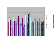
Fig 4: RNN Performance of E-Set
For E-Set, the maximum performances of speakers 1-6 are estimated as 99%, 100%, 98%, 97%, 97% & 95% respectively. For E-Set, the minimum performances of speakers 1-6 are estimated as 89%, 87%, 89%, 91%, 93% & 88% respectively. Table 2: RNN Performance of A-Set

100

RN N Performance of AH-set

I Y R

Speaker1 Speaker2 S peak er3 Speaker4 S peak er5 Speaker6

spea kers

100

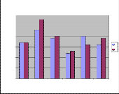
RNN Performance of A-set

J K

Fig 7: RNN Performance of AH-Set
For AH-Set, the maximum performances of speakers 1-6 are
estimated as 95%, 98%, 96%, 96%, 95% & 95% respectively.
For AH-Set, the minimum performances of speakers 1-6 are estimated as 93%, 93%, 92%, 91%, 90% & 91% respectively. Table 5: MLP Performance of E-Set

Speak er1 Speak er2 Speak er3 Speak er4 Speak er5 Speak er6

speakers

Fig 5: RNN Performance of A-Set
For A-Set, the maximum performances of speakers 1-6 are
estimated as 93%, 99%, 96%, 93%, 92% & 94% respectively.
For A-Set, the minimum performances of speakers 1-6 are estimated as 92%, 99%, 93%, 90%, 92% & 90% respectively.
Table 3: RNN Performance of EH-Set

100

MLP Performance of E-set

MLP Performance of E- Set Speaker1

MLP Performance of E- Set Speaker2

MLP Performance of E- Set Speaker3

MLP Performance of E- Set Speaker4

MLP Performance of E- Set Speaker5

MLP Performance of E- Set Speaker6

105

100

B C D E P T G V Z

speakers

Speak er1 Speak er2 Speak er3 Speak er4 Speak er5 Speaker6

speakers

Fig 6: RNN Performance of EH-Set
For EH-Set, the maximum performances of speakers 1-6 are estimated as 100%, 95%, 98%, 95%, 98% & 98% respectively.

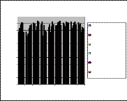
Fig 8: MLP Performance of E-Set
For E-Set, the maximum performances of speakers 1-6 are
estimated as 93%, 93%, 92%, 93%, 94% & 91% respectively.
For E-Set, the minimum performances of speakers 1-6 are
estimated as 78%, 72%, 72%, 78%, 79% & 77% respectively.
Table 6: MLP Performance of A-Set

International Journal of Scientific & Engineering Research Volume 2, Issue 6, June-2011 6

ISSN 2229-5518

100

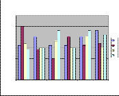
MLP Performance of AH-set

MLP Performance of A-set 70

100

60 I

50 Y

40 R

85 10

Speaker1 Speaker2 Speaker3 Speaker4 Speaker5 Speaker6

speakers

Speak er1 S peaker2 Speaker3 Speak er4 S peaker5 Speaker6

spea kers

Fig 9: MLP Performance of A-Set
For A-Set, the maximum performances of speakers 1-6 are
estimated as 87%, 98%, 90%, 83%, 90% & 89% respectively.
For A-Set, the minimum performances of speakers 1-6 are
estimated as 87%, 93%, 89%, 82%, 86% & 86% respectively.

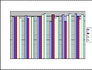
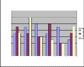
Table 7: MLP Performance of EH-Set

EH - Set	Speaker 1 %	Speaker 2 %	Speaker 3 %	Speaker 4 %	Speaker 5 %	Speaker 6 %
M	89	91	89	79	93	95
N	88	85	90	93	79	89
F	90	88	93	86	91	84
S	86	89	95	89	95	93

MLP Performance of EH-Set

100

60 M N

40 S

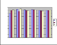
Fig 11: MLP Performance of AH-Set
For AH-Set, the maximum performances of speakers 1-6 are estimated as 92%, 95%, 92%, 93%, 90% & 91% respectively. For AH-Set, the minimum performances of speakers 1-6 are estimated as 79%, 86%, 90%, 91%, 88% & 90 % respectively.

5. TESTING PHASE

The same multilayer backpropagation algorithm is used to test the network of the spoken characters for the six speakers. Each speaker has to test the network by 18 characters repeated ten times. Each speaker, tests the word ten times and the node with the higher number in the output will be the winner node. The correct answer will be indicated by comparing this node with the input word to the network.
So by testing the characters said by each speaker the
performance can be found by the equation.
Performance = Total succeeded number of testing characters
/ Total number of characters * 100%
Table9: The performance for the test phase for each speaker.

Speaker1 % Speaker2 % Speaker3 % Speaker4 % Speaker5 % Speaker6 %

Speakers

Fig 10: MLP Performance of EH-Set
For EH-Set, the maximum performances of speakers 1-6 are estimated as 90%, 91%, 95%, 93%, 95% & 95% respectively. For EH-Set, the minimum performances of speakers 1-6 are estimated as 86%, 85%, 89%, 79%, 79% & 84% respectively.
Table 8: MLP Performance of AH-Set
The Maximum Performances of sets E, A, EH, AH are 100%,
100%, 97%, and 95% respectively. The Minimum
Performances of sets E, A, EH, AH are 75%, 80%, 77%, and
73% respectively.

CONCLUSION

This paper shows that Recurrent Neural Networks are very powerful in classifying speech signals. Even with simplified models, a small set of characters could be recognized. The performance of the nets is heavily dependent on the quality of pre-processing. Mel Frequency Cepstrum Coefficients is very reliable. Both the Multilayer Feedforward Network with backpropagation algorithm and the Recurrent Neural Network are achieving satisfying results. The results

International Journal of Scientific & Engineering Research Volume 2, Issue 6, June-2011 7

ISSN 2229-5518

obtained in this study demonstrate that speech recognition is feasible, and that Recurrent Neural Networks used are well suited for the task.

REFERENCES

[1] Ben Gold and Nelson Morgan Speech and Audio Signal
Processing, Wiley India Edition, New Delhi, 2007.
[2] B. Yegnanarayana, Artificial neural networks Prentice- Hall of India, New Delhi, 2006.
[3] John Coleman, “Introducing Speech and language processing”, Cambridge university press, 2005.
[4] Mayfield T. L., Black A. and Lenzo K., (2003).
“Arabic in my Hand: Small-footprint Synthesis of Egyptian
Arabic.” Euro Speech 2003, Geneva, Switzerland.
[5] D.A.Reynolds, “An overview of Automatic speaker
recognition technology”, proc. ICASSP 2002, orlands,
Florinda, pp.300-304.
[6] Medser L. R. and Jain L. C., (2001). “Recurrent Neural
Network: Design and Applications.” London, New York: CRC Press LLC.
[7] R.O. Duda, P.E. Hart, and D.G. Strok Pattern
Classification, 2nd edn, John Wiley, New York, 2001.
[8] Picton, P.Neural Networks, Palgrave, NY (2000).
[9] He J. and Liu L., (1999). “Speaker Verification Performance and The Length of Test Sentence.” Proceedings ICASSP 1999 vol.1, pp.305-308.
[10] Gingras F. and Bengio Y., (1998). “Handling
Asynchronous or Missing Data with Recurrent Networks.”
International Journal of Computational Intelligence and
Organizations, Vol. 1, no. 3, pp. 154-163
[11] Jihene El Malik, (1998). “Kohonen Clustering Networks
For Use In Arabic Word Recognition System.” Sciences
Faculty of Monastir, Route de Kairouan, 14-16 December.
[12] RuxinChenand Jamieson L. H., (1996). “Experiments on the Implementation of Recurrent Neural Networks for Speech Phone Recognition.” Proceedings of the Thirtieth Annual Asilomar Conference on Signals, Systems and Computers, Pacific Grove, California, November, pp.
7790782.
[13] Koizumi T., Mori M., Taniguchi S. and Maruya M., (1996). “Recurrent Neural Networks for Phoneme Recognition.” Department of Information Science, Fukui University, Fukui, Japan, Spoken Language, ICSLP 96, Proceedings, Fourth International Conference, Vol. 1, 3-6
October, Page(s): 326 -329.
[14] Joe Tebelskis, (1995). “Speech Recognition using Neural
Network.”Carnegie Mellon University: Thesis Ph.D.
[15] C.M.Bishop, Neural Networks for pattern recognition,
oxford university press, 1995.
[16] Rabiner, L and Juang, B, -H; fundamentals of speech recognition, PTR prentice Hall, scan Francisco, N.J (1993). [17] Lee S. J., Kim K. C., Yoon H. and Cho J. W., (1991). “Application of Fully Neural Networks for Speech Recognition.” Korea Advanced Institute of Science and Technology, Korea, Page(s): 77-80.
[18] Werbos P., (1990). “Backpropagation Through Time: What It Does and How To Do It.” Proceedings of the IEEE,
78, 1550.
[19] Lippman R.P., (1989). “Review of Neural Network for
Speech Recognition.” Neural Computation 1.1-38.