International Journal of Scientific & Engineering Research, Volume 4, Issue 9, September-2013 2604

ISSN 2229-5518

Solution of Second Order Ordinary Differential Equation with Periodic

Solutions

*O. M. Akinmoladun(1) , R. A. Ademiluyi(2), A. A. Abdurasid(3) and D. A. Farinde(4)

1,3,4 Department of Mathematics & Statistics, Lagos-State Polytechnics, Ikorodu, Lagos, Nigeria

,2,Department of Mathematical Sciences, Federal University of Technology, Akure, Nigeria., , Correspondence author: +2348038727249*, email: olusegun_m@yahoo.com*

Abstract

In this paper, a discrete Implicit Linear Multistep Method (LMM) of Direct Solution of IVP second order

ordinary differential equation with periodic solution was developed at step length k = 3, using trigonometric function as a basis function. The computational burden and computer time wastage involved in the usual reduction of second order problem into system of first order equations are avoided

by this method. The development of the method adopts Taylor series expansion techniques and Boundary Locus stability test method. The developed method was found to be accurate, consistent, zero stable, P- stable and convergent. The method was used to solve sample problem on second order ordinary differential equation with periodic solutions and results are quite suitable when compared with other existing methods.

Key Words; Oscillatory, Periodic, LMM, ODE, Stability, Trigonometry, Taylor series

1.0.0 INTRODUCTION

Any function of the form

y’’ = f(t, y) a ≤ t ≤ b, y(a) = y0 , y′(a) = α (1.0.1)

where f(t + T, y) = f(t, y) where T is the period.

is called initial value problems of second order ordinary differential equation with periodic solution. Solutions to the IVP of the type (1.0.1) are highly oscillatory in nature and thus severely restrict the

conventional linear multistep method of such system which often occurs in mechanical system without dissipation, satellite tracking and celestial mechanics [[7], [9], [3]]

One of the conditions that such equation (1.0.1) must be satisfied in order to ensure the existence and

uniqueness of solution is contained in theorem postulated by [5].

According to [7], [8], [12], and [10] ; the commonest method of solving a second order ordinary differential equation of the form (1.0.1) is by reduction of the problem into first ordinary differential equation.

However, a more serious drawback to such technique arises when the given system of equations to be solved cannot be solved explicitly for the derivatives of the highest order and, thereby; become inefficient, uneconomical for a general purpose application.

In this work, a discrete Linear Multistep Method of the form

𝑘−1

k−1

𝑦𝑛+𝑘 = � 𝑎𝑗 𝑦𝑛+𝑗 + (ℎ)2 � 𝛽𝑗 y′′

𝑛+𝑗

(1.0.2)

𝑗=0

𝑗=0

is developed at step length K = 3 ; for direct solution of second order initial value problems of ordinary differential equation of the form (1.0.1) using trigonometric function as a basis function

IJSER © 2013 http://www.ijser.org

International Journal of Scientific & Engineering Research, Volume 4, Issue 9, September-2013 2605

ISSN 2229-5518

2.0 DERIVATION OF THE METHODS

The development of the numerical methods for solution of periodic initial value problems of ordinary differential equation of the form

y|| = f(t, y) a ≤ t ≤ b, y(a) = y0, y′(a) = α 2.0.0 where f(t + T, y) = f(t, y) where T is the period.

Assuming the theoretical solution of the equation (2.0.0) is of the form

y(t) = a cos wt + b sin wt 2.0.1

At, t = tn

yn = y(tn) = a cos wtn + b sin wtn 2.0.2

y1(tn ) = y1 n = a w sin wtn + bw cos wtn

y11(tn) = y11 n = - w2 (a cos wtn + b sin wtn ) = fn 2.0.3

fn = - w2yn 2.0.4

tn+k = tn + kh where k = 0, 1, 2, 3, 4.and h = tn+1 - tn 2.0.5

Similarly,

At t = tn+1

y(tn+1) = yn+1 = a cos wtn+1 + b sin wtn+1 2.0.6 y1(tn+1 ) = y1 n+1 = awsin wtn+1 + bwcos wtn+1 2.0.7 y11(tn+1) = y11 n+1 = -w2 (a cos wtn+1 + b sin wtn+1)

fn+1 = - w2yn+1 2.0.8

At t = tn+2

y(tn+2) = yn+2 = a cos wtn+2 + b sin wtn+2 2.0.9 y1(tn+2 ) = y1 n+2 = w a sin wtn+2 + bw cos wtn+2 2.0.10 y11(tn+2) = y11 n+2 = -w2 (a cos wtn+2 + b sin wtn+2) = fn+2 2.0.11 fn+2 = - w2yn+2 2.0.12

At t = tn+3

y(t) = y(tn+3) = yn+3 = a cos wtn+3 + b sin wtn+3 2.0.13 y1(tn+3 ) = y1(tn+3 ) = y1 n+3 = w a sin wtn+3 + bw cos wtn+3 2.0.14 y11(tn+3) = y11(tn+3 ) = y11 n+3 = w2 (a cos wtn+3 +b sin wtn+3) = fn+3

2.0.15

fn+3 = - w2yn+3 2.0.16

2.1 METHODOLOGY

Subtracting equation (2.0.9) from equation (2.0.13) to get

yn+3 - yn+2 = a(cos wtn+3 – cos wtn+2 ) + b (sin wtn+3 – sin wtn+2 ) 2.1.1

By adopting trigonometric difference equation method and simplifying to obtain

wh  w w 

yn+3 – yn+2 = - 2 sin

2 a sin

(2t + 5h) + b cos (2t + 5h)

2 2 

2.1.2

Subtract equation (2.0.15) from (2.1.2) to obtain;

yn+3 – 2yn+2 + yn+1 = -4 sin2 [a cos w (t

2 n

+ 2h) + b sin w (t n

+ 2h)]

2.1.3

Subtract 2. 0.16 from 2.1.3 to obtain:

 wh   w w 

2.1.4

yn+3 – 3yn+2 +3yn+1 –yn = -8sin3 

 2

Add equation (2.0.3) and (2.0.8)

 a cos

 

(2t n

2

+ 3h) + b sin

(2t n

2

+ 3h)



IJSER © 2013 http://www.ijser.org

International Journal of Scientific & Engineering Research, Volume 4, Issue 9, September-2013 2606

ISSN 2229-5518

wh

f n+1 + f n = - 2 w2 cos

2

�𝑎𝑐𝑜𝑠

2 (2𝑡𝑛

+ 3ℎ) + 𝑏𝑠𝑖𝑛

2 (2𝑡𝑛

+ 3ℎ)� 2.1.5

Add equations (2.0.15) and (2.0.11) to obtain;

wh

f n+3 + f n+2 = - 2 w2 cos

2



a cos

w (2t

2 n

+ 5h) + b sin

w (2t

2 n

+ 5h)



2.1.6

Similarly adding equation 2.1.5 to 2.1.6 and simplify to get

wh

f n+3 + 2f n+2 + f n+1 = - 4w2 cos2 [a cos w (t

2 n

+ 2h) + b sin w (2t n

+ 2h)]

2.1.7

In the same way; add equation 2.1.7 to equation 2.1.5 and simplify to get

wh  w w 

f n+3 + 3f n+2 +3f n+1 + f n = - 8w2 cos3 a cos

(2t n

+ 3h) + b sin

(2t n

+ 3h)

2.1.8

2  2 2 

Divide equation (2.1.4) by equation (2.1.7) to obtain

3

n +3 − 3 n + 2 + 3 n +1 − n

= 1  tan 

2.1.9

y y y

y  wh 

f n +3

+ 3 f

n + 2

+ 3 f

n +1

+ f n

w 2  2 

Using Taylor’s series expansion to simplify equation (2.1.9) to obtain

y − 3 y

+ 3 y − y

1  1

w2 h 2

w4 h 4 

n +3 n + 2 n +1 n

=  +

+ + ....

2.1..10

f n +3

+ 3 f

n + 2

+ 3 f

n +1

+ f n

2  24

240 

Assuming h is sufficiently small such that wh is also small, then (2.1.10) modifies into

h 2

yn+3 – 3yn+2 + 3yn+1 – yn =

2 3

h 2

(f n+3 + 3f n+2 +3f n+1 + f n ) 2.1.11

yn+3 = 3yn+2 - 3yn+1 + yn +

8

3.0 Definition

(f n+3 + 3f n+2 +3f n+1 + f n ) 2.1.12

Let П (r, h) = ρ(r) – h δ(r) (3.1.0)

denotes the characteristic polynomial equation of the method where ρ(r) and δ (r) are called first and

second characteristics polynomials respectively; as explained by [11].

In the spirits of [4], [10], [15], [12] [13], [14]; a linear multistep method is said to be consistent if and only if it satisfies the following conditions

(i ) The

k

order

P ≥ 1 



(ii ) ∑αj = 0 

j =0 

1 

. (.3.1.1)

(iii )

ρ (r ) = ρ

(r ) = 0

(iv) ρ 11 (r ) = 2 ! δ (r ) 

With the principal root r ≤ 1

from (3.2.1) the characteristic polynomial equation of the 2-step method (1.2.14) is

𝑟3 + 3𝑟2 + 3𝑟 + 1 = 1 (𝑟3 +3𝑟2 + 3𝑟 + 1)

8

where ρ(r) = 𝜌(𝑟) = 𝑟3 − 3𝑟2 + 3𝑟 − 1 ; 𝑎𝑛𝑑 𝛿(𝑟) = 1 (𝑟3 +3𝑟2 + 3𝑟 + 1)

8

Simplifying equation (3.2.3), we have (r – 1)(r – 1)(r-1) = 0, r = 1, 1,1

Thus, ρ(1) = 0 = ρ/(1), 𝜌′′ |1| = 0 = 2! 𝛿|−1|

𝑘

𝑗=0

α𝑗 = 1 − 3 + 3 − 1 = 0

IJSER © 2013 http://www.ijser.org

International Journal of Scientific & Engineering Research, Volume 4, Issue 9, September-2013 2607

ISSN 2229-5518

Therefore the method (2.1.12) is consistent, convergent and zero stable.

3.2.0 STABILITY PROPERTIES OF THE METHOD

A linear multistep method of the form (1.0.2) is said to be

(i) Zero stable if no root of the first characteristics polynomial has modulus greater than one that is it

must be within a unit circle.

(ii) Absolutely or relatively stable in a region R of the complex plane if for all h ∈ R; all roots (rs ) of the stability polynomial π(r, h ) associated with the method satisfy.

| rs | < | ; s = 1, 2, …. K, ∀ |rs | < | r1 |

S = 2, 3, 4….., k, [ according to [11], [ 5]] (3.2.1)

REGION OF ABSOLUTE STABILITY

The method in equation (2.1.12) satisfies the conditions for zero stability since there is no root of its first

characteristic polynomial ρ(r) that is greater than one since

ρ(r) = r3 – 3r2 + 3r – 1 = 0 3.4.2 (r – 1)(r – 1)(r – 1) = 0, r = 1, 1, 1

To test for region of absolute stability; the following steps can be followed;

h (r ) =

T (r )

H (r ) =

8(r 3 − 3r 2 + 3r − 1)

r 3 + 3r 2 + 3r + 1

3.4.3

Let r = ei θ = Cos θ + i sin θ 3.4.4

T(r) = [32 cos3 θ – 48 cos2 θ – 4] + i [6sinθ cos θ + 3sin θ]

H(r) = [4 cos3 θ + 6 cos2 – 2] + i [6sinθ cos θ + 3sin θ] 3.4.5

h (θ )= X (θ )+ i Y (θ )

( ) (32 cos3 θ − 48 cos 2 θ − 4)(4 cos3 θ + 6 cos 2 θ − 2)+ (6 sin θ cosθ

+ 3 sin θ )2

3.4.6

X θ =

(4 cos3 θ + 6 cos 2 θ − 2)2 + (6 sin θ cosθ

+ 3 sin θ )2

( ) (6 sin θ cosθ + 3 sin θ )(− 28 cos3 θ + 53 cos 2 θ + 2)

Y θ =

(4 cos3 θ + 6 cos 2 θ − 2)2 + (6 sin θ cosθ

+ 3 sin θ )2

where X(θ) was evaluated for values of θ ranges between 00 and 1800 and the results ere tabulated below

Table 2

That is, its region of absolute stability is within interval (-45, -∞). It is P-Stable.

4.0 NUMERICAL EXPERIMENTS

4.1 SAMPLED PROBLEMS

y11 = - y
Y1(0) = 1, y(0) = 0
Theoretical Solution y(x) = Sin X
For implementation of the developed method in solving the sampled problem, FORTRAN programs were developed at step size h = 0.1, 0.01 and 0.001 and computerized for steps k = 3. The performance of the method on the sampled problem was shown below in tabular and graphical forms.

IJSER © 2013 http://www.ijser.org

International Journal of Scientific & Engineering Research, Volume 4, Issue 9, September-2013 2608

ISSN 2229-5518

PERFORMANCE OF PROPOSED METHOD ON SAMPLE PROBLEM

Where Step k = 3 and h = 0.1

IJSER © 2013 http://www.ijser.org

International Journal of Scientific & Engineering Research, Volume 4, Issue 9, September-2013 2609

ISSN 2229-5518

TABLE 2B: PERFORMANCE OF PROPOSED METHOD ON THE SAMPLE PROBLEM

Where Step k = 3 and h = 0.01

IJSER © 2013 http://www.ijser.org

International Journal of Scientific & Engineering Research, Volume 4, Issue 9, September-2013 2610

ISSN 2229-5518

TABLE 2C: PERFORMANCE OF PROPOSED METHOD ON THE SAMPLE PROBLEM

Where Step k = 3 and h = 0.001

IJSER © 2013 http://www.ijser.org

International Journal of Scientific & Engineering Research, Volume 4, Issue 9, September-2013 2611

ISSN 2229-5518

FIGURE 2A: GRAPH SHOWING EXACT SOLUTION, NUMERICAL RESULT OF THE SAMPLE PROBLEM

where k = 3 and h = 0.1

3.00000

2.00000

1.00000

0.00000

-1.00000

-2.00000

-3.00000

NUMERICAL RESULT EXACT SOLUTION

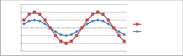
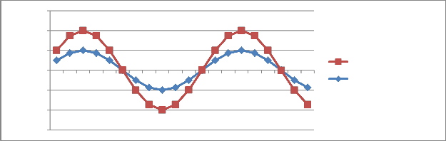
FIGURE 2B: GRAPH SHOWING EXACT SOLUTION, NUMERICAL RESULT OF PROBLEM 1 where k = 3 and h = 0.01

3.00000

2.00000

1.00000

0.00000

-1.00000

NUMERICAL RESULT EXACT SOLUTION

-2.00000

-3.00000

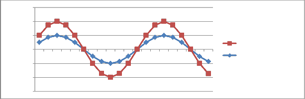
FIGURE 2C: GRAPH SHOWING EXACT SOLUTION, NUMERICAL RESULT OF PROBLEM 1 where k = 3 and h = 0.001

3.00000

2.00000

1.00000

0.00000

-1.00000

NUMERICAL RESULT EXACT SOLUTION

-2.00000

-3.00000

1.5.0 CONCLUSION

IJSER © 2013 http://www.ijser.org

International Journal of Scientific & Engineering Research, Volume 4, Issue 9, September-2013 2612

ISSN 2229-5518

In this work, numerical method for solution of periodic initial value problems of second order ordinary differential equation had been discussed. The developed method was analyzed and found to be consistent, convergent and stable.
The performance of the method was implemented on some sampled problems of second order ordinary differential equation with oscillatory solutions. The results show that as the values of h decreases from 0.1 to 0.001, the
truncation error approaches zero. It was also observed that as h decreases the graph of the numerical result (NR) and the exact solution (ES) of the proposed methods at each steps of k were nearly overlaps each other and the discretization error vanishes as h tend to zero, showing that the proposed method is accurate and can compare favourably with the result on table 2.

REFERENCES

1. Ademiluyi, R.A. (1987) “ New hybrid methods for system of stiff ordinary differential equation” Ph.D thesis, University of Benin, Benin-City, Nigeria. (unpublished)
2. Ademiluyi, R.A. and Kayode, S.J. (2001) Maximum order second derivative hybrid multistep methods for
integration of initial value problems in ordinary differential equations” Journal Nig. Ass. Math Phy Vol. 5, pp254 – 262
3. Akinmoladun O.M. (2011) Solution of Second Order Ordinary Differential Equations with Oscillatory Solution
An M.Tech. Thesis submitted to The Federal University of Technology,, Akure, Nigeria. July,
2011.(Unpublished)
4. Awoyemi, D.O. (1999): “A class of continuous methods for general second order initial value problems of
ordinary differential equations” Journal of the Mathematical Association of Nigeria, Vol. 24, 162, pp 40-43
5. Codington, E.A. and Levinson, N. (1955):
Theory of ordinary differential equations McGraw – Hill, New-York
6. Dahlquist, G. (1969) “ A Numerical Method for some ODEs with large Lipschitz & constants” information processing 68, North Holland Publishing company, Amsterdam.
7. Fatunla S.O. (1988) ‘’Numerical methods for IVPs in ordinary differential equations’’. Academic press Inc.
Harcourt Brace Jovano. Publishers New York.
8. Fatunla S.O. (1992) ‘’ Parallel methods for second order ODE’s’’ Computational ordinary differential
equations proceedings of comp. conference (eds),pp 87-pp 99
9. Henrici, P. (1962): Discrete variable methods in ordinary Differential equations John Wiley and sons, New
York.
10. Jain et. al. (1984) “A sixth order p-stable symmetric multistep method for periodic initial value problems of second order differential equation” IMA Journal on Numerical Analysis. vol. 4 pp 117 - 125
11. Kayode S.J. (2004) “A class of maximal order Linear collocation methods for direct solution of second order initial value problems ordinary differential equations” Ph.D. thesis, FUTA , Nigeria. (unpublished).
12. Lambert J.D. (1973) “computational method in ordinary differential equations” John Willey and sons Inc New
York
13. Lambert J.D. (1980) “Stiffness” proceeding computational Techniques for ordinary differential equation (Gladwell I and Sayers D.K. ed) 1946 Academic press a subsidiary of Harcurt Brace Jovanovich publishers London, New York Toronto Sydney San Francisco.
14. Lambert J.D. (1991) “Numerical methods for ordinary differential system of initial value problems” John
Willey and sons Inc, New-York.
15. Onumanyi P., Awoyemi D. O., Jator S. N. and Sirisena U. W. (1994) New Linear multistep methods with continuous coefficients for the first order initial value problems. J. Nig. Math. Soc. Vol. 13, pp 37-51

IJSER © 2013 http://www.ijser.org