International Journal of Scientific & Engineering Research, Volume 5, Issue 2, February-2014 885
ISSN 2229-5518
Sample Based Curve Fitting Computation on the
Performance of Quicksort in Personal Computer
Dipankar Das, Arijit Chakraborty, Avik Mitra
Abstract— In this paper we have used curve fitting technique for analyzing the classical Quicksort algorithm and its performance in worst case on personal computer. The proposed generic model can be viewed as: Time ~ f (Number of Elements). We fit the data points (Time vs Number of elements) in twenty one different models from various types of fit such as Polynomial, Exponential, Power, Gaussian and Fourier. This analysis leads us to identify the best model amongst these models. We found that a model of Fourier series is the best fit.
Index Terms— Curve Fitting, Experimental Algorithmics, Fourier Fit, Graphical Residual Analysis, Performance Analysis, Quicksort, Worst
Case
—————————— ——————————
OMPUTATIONAL experiments on the performance of algorithms give us further insight into their behaviors in real world scenarios and supplement their theoretical
analysis. Algorithmic work and experimentation are combined in Experimental algorithmics [1].
There is a trend in research community to measure perfor- mance of complex algorithms by employing various models. The situation is not different for common sorting algorithms as well; curve fitting gives us visual information to look upon the situation in a subtle way, based on the motivation of easily available computing devices like personal computers, laptops etc and softwares like GCC, MATLAB etc.
Performance analysis of Quicksort which is one of the pop- ular sorting algorithms [2] in a simulated environment will give us a fair idea about various dimensions of the algorithm.
There are two ways of analyzing Quicksort algorithm [34] by
C.A.R. Hoare.
Theoretical [3], [4], [5], [6], [7], [8], [9], [10], [11], [12],
[13]
Empirical [14], [15], [16]
Theoretical analyses are done with respect to the following
parameters:
Run-time [3], [4], [5]
Probabilistic distribution on the number of compari-
sons required during sorting [7], [9]
The limit theorem on the distribution [8], [10], and
————————————————
• Arijit Chakraborty is currently working as a Faculty member in The Herit-
age Academy, Kolkata, India, PH-919830722218. E-mail:
arijitchakraborty.besu@gmail.com
• Avik Mitra is currently working as a Faculty member in The Heritage
Academy, Kolkata, India, PH-918902727029. E-mail:
avik.mitra2@gmail.com
deviations from that limit for finite number of ele- ments [11], [12].
Empirical analyses are based on the response time of Quicksort to patterns (i.e. already arranged, partially ar- ranged, reverse arranged) in the list of elements that is to be sorted i.e. adaptive ability [14] of Quicksort.
Analyses of variations [15] of Quicksort like Qsorte [25], qsort7 [26] etc are based on:
Number of comparisons and swaps required during running of Quick sort [14], [15].
Comparative analysis of pivoting schemes [14], [15].
Affect of computer configuration like type of micro-
processor, L1 cache miss events, and branch miss-
predictions by the microprocessors etc [14].
Several developments of Quicksort have been performed. These developments include how well the Quicksort be tuned for parallel processing environment like distributed memory system [19], graphics processing unit [18], or online version of Quicksort [20]; in the online version of Quicksort, called Quick sort on the fly, the first element in the sorted arrangement is found and put in the output before the rest of the elements are sorted, thus, the output appears as a stream. A generalization of Quicksort has also been explored where respective the au- thors proposed a solution of the problem of sorting by consid- ering the first k largest elements in a set of n elements [24].
Other types of developments include proposals for new single pivot selection schemes [21], [22], and multiple pivot selection schemes [21], [23]; in [23] three pivots are considered for reducing the run-time of Quicksort in average case.
We tried to identify the best curve that can be fitted to the data points (Time vs Number of elements) generated by simulating Quicksort algorithm for the worst case.
The objective of this study is to propose a generic mathe- matical model using large dataset that can explain the behav- ior of Quicksort for worst case in a personal computer.
IJSER © 2014 http://www.ijser.org
International Journal of Scientific & Engineering Research, Volume 5, Issue 2, February-2014 886
ISSN 2229-5518
Open source platform and ANSI C have been used to generate the experimental data. The sample data set is given in the fol- lowing table (TABLE 1):
TABLE 2
POLYNOMIAL MODEL EXPRESSIONS IN MATLAB
TABLE 1
SAMPLE DATA POINTS
In this case, the researchers have chosen ‘Time’ as the response (dependent) variable and ‘Number of elements’ as the predic- tor (independent) variable for analyzing the data.
Thus the proposed generic model can be written as: ![]() (1)
(1)
The data points have been fitted with twenty one different
types of models from different types of fit (Polynomial, Expo-
nential, Gaussian, Power and Fourier) and the goodness of fit statistics of these models are calculated.
The model expressions of these models have been tabulated below in the following tables (TABLE 2 – TABLE 6):
IJSER © 2014 http://www.ijser.org
TABLE 3
EXPONENTIAL MODEL EXPRESSIONS IN MATLAB
TABLE 4
POWER MODEL EXPRESSIONS IN MATLAB
![]()
TABLE 5
GAUSSIAN MODEL EXPRESSIONS IN MATLAB
International Journal of Scientific & Engineering Research, Volume 5, Issue 2, February-2014 887
ISSN 2229-5518
TABLE 6
FOURIER MODEL EXPRESSIONS IN MATLAB
In this study all the curve fitting has been performed using
‘Non linear least square’ [35] method, keeping ‘Robust’ [36]
off. The researchers have used ‘Trust-Region’ [37] algorithm
for curve fitting. The entire analysis was performed at 95%
confidence level.
For the purpose of this study the following goodness of fit statis- tics have been considered:
a. R2
b. Adjusted R2
c. Sum of squares due to error (SSE)
d. Root mean squared error (RMSE)
A better fit is indicated by high value of R2 and Adjusted R2
(value close to 1). Similarly, low value of SSE and RMSE (val-
ue close to 0) also indicate a better fit [27].
The best model is chosen based on highest R2 and Adjusted R2 value (close to 1) and lowest values of SSE and RMSE (close to 0).
In statistical modeling residual analysis plays an important role. The quality of a regression can be assessed by using re- sidual plots [28].
Residual is defined as:
Residual = observed value – predicted value
In general residuals are a form of errors and the same gen- eral assumptions of errors can be applied to the residuals too. It is expected that the residuals should be (roughly) normal and (approximately) independently distributed with a mean of 0 and some constant variance [29].
In this study, the following graphical residual analysis methods have been used to assess the quality of regression:
a. Residual vs predictor plot b. Residual plot
c. Residual lag plot
d. Histogram of the residuals
e. Q-Q plot of the residuals
To assess sufficiency of the functional part of the model this plot is used. If the residuals in the plot do not exhibit any sys- tematic structure then it indicates that the model fits the data well [30].
This plot is used to check the error variance. If the residual plot has an increasing/ decreasing trend then it indicates that the error variance increases/ decreases with the independent variable. A horizontal-band pattern indicates that the variance of the residuals is constant [28].
This plot is used for checking the independence of the error term. It is a scatter plot of residuals (i) on the y axis and the residual (i-1) values on the x axis. Any random pattern in a lag plot suggests that the variance is random [28]. If there is no pattern or structure in the plot i.e. the points appear to be ran- domly scattered then it suggests that the errors are independ- ent [31].
This is test for residual normality. A symmetric bell shaped his- togram which is evenly distributed around zero suggests that the residuals are normally distributed [32].
A Q-Q plot is a probability plot. It is a graphical method for
comparing two probability distributions by plotting their
quantiles against each other. If the points on the plot are linear
then it suggests that the randomly generated data are normal-
ly distributed [33].
We have used Fedora 14 (Kernel Version 2.6), ANSI C for generating experimental data and for the purpose of the data analysis of this paper MATLAB 7.7.0, SPSS 17.0 and MS Excel have been used.
IJSER © 2014 http://www.ijser.org
International Journal of Scientific & Engineering Research, Volume 5, Issue 2, February-2014 888
ISSN 2229-5518
The Quicksort algorithm has been executed and simulated in a hardware platform which is as follows:
Processor: Intel Core 2 Duo CPU T6570 @2.10 GHz
RAM: 3GB; DDR-3; frequency-399.0 MHz
L1 Data Cache Size: 32 KB (8-way set associative)
L1 Instruction Cache Size: 32 KB (8-way set associa-
tive)
L2 Cache size: 2048 KB (8-way set associative)
The twenty one fitted models are first evaluated using the goodness of fit statistics and the best model amongst the fitted models has been identified based on the decision rule as dis- cussed in sub section 4.3.
A summary of goodness of fit statistics is given in TABLE 7.
TABLE 7
GOODNESS OF FIT STATISTICS
Φ Best model.
# Equation is badly conditioned.
§ Fit computation did not converge.
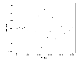
Fig. 1. Residual vs predictor plot of Fourier7 model.
From the above figure (Fig. 1.) it is evident that the residu- als appear to behave randomly. Therefore, it suggests that the model fits the data well.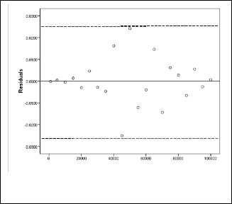
Fig. 2. Residual plot of Fourier7 model.
We can find a horizontal band pattern from the above fig- ure (Fig. 2.) which suggests that the variance of the residuals is constant and the regression is a good one.
In this subsection the graphical residual analysis of the best mod- el (identified in sub section 5.1) has been performed.
IJSER © 2014 http://www.ijser.org
International Journal of Scientific & Engineering Research, Volume 5, Issue 2, February-2014 889
ISSN 2229-5518
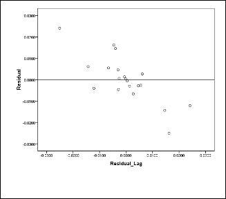
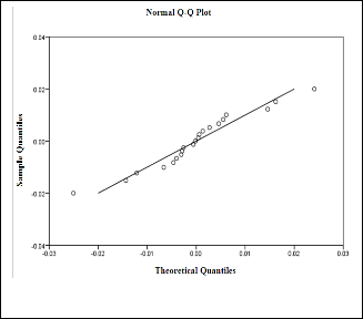
Fig. 3. Residual lag plot of Fourier7 model.
Fig. 5. Q-Q plot of the residuals of Fourier7 model.
The random pattern in the lag plot (Fig. 3.) suggests that the variance is random and it suggests that the errors are inde- pendent.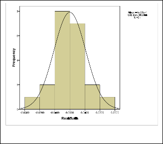
Fig. 4. Histogram of the residuals of Fourier7 model.
The above figure (Fig. 4.) exhibits a symmetric bell shaped histogram which is evenly distributed around zero. Therefore it suggests that the residuals are normally distributed.
It may be easily observed from the figure (Fig. 5.) that the residuals are approximately linear. Therefore it suggests that the residuals follow approximately normal distribution.
From the subsection 5.2 the residuals appear to be randomly distributed around zero. Hence, it can be suggested that the model appear to fit the data well and it can be concluded that
‘Fourier7’ model is the best fit in this case.
The proposed mathematical model is given below:
Here, the value of ‘w’ is equal to 0.0000486. The plot of the proposed model is shown in Fig. 6. The circles indicate data points and the solid line represents the curve of the proposed model.
IJSER © 2014 http://www.ijser.org
International Journal of Scientific & Engineering Research, Volume 5, Issue 2, February-2014 890
ISSN 2229-5518
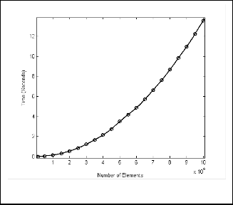
Fourier type of fit. The study shows that among the various available models, the Fourier type of models may be explored in depth while analyzing the performance of Quicksort in worst case.
Fig. 6. Proposed model (Fourier7).
We ran classical Quicksort algorithm on a particular machine configuration i.e. hardware and a state of the operating sys- tem. We are yet to explore the effects of different hardwares and operating system configurations and its states on the per- formance of Quicksort in worst case.
We have also not considered factors pertained to operating system (Fedora 14 in this case) i.e. context switch time, cache hit, cache miss, buffering etc.
Various pivoting schemes also are not explored in this pa- per.
It will certainly be our future endeavor to consider these factors as we believe that these factors can contribute to actual execution time of Quicksort.
This article is a simplistic representation of the said algo- rithm, hence we assumed the net iteration time to be our exe- cution time, but in reality the total execution time of the algo- rithm is higher though in negligible proportion.
In this study we have used curve fitting techniques to examine the experimentally simulated dataset. After plotting the da- taset given in TABLE 1 (Number of elements in X axis and Time in Y axis), it is evident that the dataset has a definite pat- tern and takes a shape of a curve i.e. it is following curvilinear- ity. The data have been analyzed by using different type of fits namely Polynomial, Exponential, Power, Gaussian and Fouri- er. The analysis shows that the Fourier type of fit outper- formed all the other types of fit in terms of goodness of fit sta- tistics. In this case, ‘Fourier7’ is the best fit with highest R2 (0.999994), highest Adjusted R2 (0.999976), lowest SSE (0.0022) and lowest RMSE (0.0212). Graphical residual analysis of Fou- rier7 model exhibits that the model fits the data well, variance of the residuals is constant, errors are independent, residuals are normally distributed and approximately linear. This indi- cates that the performance of Quicksort in worst case follows
[1] R. Fleischer, B. Moret and E.M. Schmidt, eds., Experimental Algorith- mics From Algorithm Design to Robust and Efficient Software, Berlin, Heidelberg: Springer-Verlag, pp. V, 2002.
[2] T. Niemann, “Sorting and Searching Algorithms,” http://epaperpress.com/sortsearch/download/sortsearch.pdf. (Ac- cessed November, 2013).
[3] I. Parberry, “Analysis of Quicksort”, Technical Report, Department of Computer Science, University of North Texas, 1997.
[4] M. Fouz, M. Kufleitner, B. Manthey, N.Z. Jahromi, “On Smoothed Analysis of Quicksort and Hoare’s Find”, Algorithmica, Vol. 62, Is- sue3-4, pp 879-905, April 2012.
[5] R. Sedgewick, “Implementing Quicksort Programs”, Communications of the ACM, Vol. 21, Issue 10, October 1978.
[6] U. Rosler, “A Limit Theorem for Quicksort”, Theoretical Informatics and Applications, Vol. 25, Issue 1, pp 85-100, 1991.
[7] C.J.H. McDiarmid, R.B. Hayward, “Large Deviations for Quicksort”,
Journal of Algorithms, Vol. 21, Issue 3, pp 476-507, November 1996.
[8] J.A.Fill, S. Janson, “Approximating The Limiting Quicksort Distribu- tion”, Random Structures and Algorithms, Vol. 19, Issue 3-4, pp 376-406, December 2001.
[9] M. Fuchs, “A Note on the Quicksort Asymptotics”, Random Structures and Algorithms, November 2013, doi: 10.1002/rsa.20524.
[10] R. Neininger, “Refined Quicksort Asymptotics”, Random Structures and Algorithms, April 2013, doi: 10.1002/rsa.20497.
[11] J.A. Fill, “Distributional Convergence for the Number of Symbol Comparisons Used by Quicksort”, The Annals of Applied Probability, Vol. 23, No. 3, pp 859-1289, 2013.
[12] S. Wild, M.E. Nebel, “Average Case Analysis of Java 7’s Dual Pivot Quicksort”, Proceeding of the 20th Annual European Conference on Algo- rithms, pp 825-836, 2012.
[13] J.A. Fill, S. Janson, “Smoothness and Decay Properties of the Limiting
Quicksort Density Function”, Trends in Mathematics, pp 53-64, 2000. [14] G.S. Brodal, R. Fagerberg, G. Moruz, “On the Adaptiveness of Quick-
sort”, ACM Journal of Experimental Algorithmics, Vol. 12, Article No.
3.2, 2008.
[15] L. Khreisat, “Quicksort: A Historical Perspective and Empirical
Study”, IJCNS, Vol. 12, No. 12, December 2007.
[16] S.F. Solehria, S. Jadoon, “Multiple Pivot Sort Algorithm is Faster than Quicksort Algorithm: An Empirical Study”, International Journal of Electrical and Computer Sciences, Vol. 11, No. 3, June 2011.
[17] H. Erkio, “The Worst Case Permutation for Median-of-Three Quick- sort”, The Computer Journal, Vol. 27, No. 3, 1984.
[18] D. Cederman, P. Tsigas, “GPU-Quicksort: A Practical Quicksort Al- gorithm for Graphics Processors”, ACM Journal of Experimental Algo- rithmics, Vol. 14, Article No. 4, 2009.
[19] P. Sanders, S. Peter, T. Hansch, “On the Efficient Implementation of Massively Parallel Quicksort”, Solving Irregularly Structured Problems in Parallel, pp13-24, 1997.
[20] M. Ragab, U. Roeslar, “The Quicksort Process”, Stochastic Processes and Their Applications, Vol 124, Issue 2, pp 1036-1054, February 2014.
[21] K.C. Kiwiel, “Partitioning Schemes for Quicksort and Quickselect”,
The Computing Research Repository, Vol. 312054, 2003.
IJSER © 2014 http://www.ijser.org
International Journal of Scientific & Engineering Research, Volume 5, Issue 2, February-2014 891
ISSN 2229-5518
[22] A. Mohammed, M. Othman, “A New Pivot Selection Scheme for
Quicksort Algorithm”, Journal of Science and Technology, Vol. 11, pp
211-215, 2004.
[23] S. Kushagra, A.L. Ortiz, A. Qiao, J. Ian Munro, “Multi-Pivot Quick- sort: Theory and Experiments”, Proceedings of the 16th Workshop on Algorithm Engineering and Experiments (ALENEX), pp 47-60, 2014.
[24] S.H. Shiau, C.B. Yang, “The Generalization of Quicksort”, Proceedings of Workshop on Internet and Distributed Systems (WIND), 2000.
[25] R.L. Wainright, “Quicksort Algorithms with an Early Exit for Sorted Subfiles”, Proceedings of the 15th Annual Conference on Computer Sci- ence, pp 183-190, 1987.
[26] J.L. Bentley, M.D. Mcllroy, “Engineering a Sort Function”, Software: Practice and Experience, Vol. 23 (11), pp 249-265, November 1993.
[27] Evaluating Goodness of Fit – MATLAB & Simulink – MathWorks India, MathWorks, [online], http://www.mathworks.in/help/curvefit/evaluating-goodness-of- fit.html (Accessed: November, 2013).
[28] Graphic Residual Analysis, OriginLab, [online], http://www.originlab.com/www/helponline/origin/en/UserGuid e/Graphic_Residual_Analysis.html (Accessed: November, 2013).
[29] 5.2.4. Are the model residuals well-behaved?, Engineering Statistics Handbook, [online], http://www.itl.nist.gov/div898/handbook/pri/section2/pri24.htm (Accessed: November, 2013).
[30] 4.4.4.1. How can I assess the sufficiency of the functional part of the model?, Engineering Statistics Handbook, [online], http://www.itl.nist.gov/div898/handbook/pmd/section4/pmd441
.htm (Accessed: November, 2013).
[31] 4.4.4.4. How can I assess whether the random errors are independent from one to the next?, Engineering Statistics Handbook, [online], http://www.itl.nist.gov/div898/handbook/pmd/section4/pmd444
.htm (Accessed: November, 2013).
[32] Normal Probability Plot of Residuals | STAT 501 – Regression Methods, PENNSTATE, [online], https://onlinecourses.science.psu.edu/stat501/node/40 (Accessed: November, 2013).
[33] G. Bandyopadhyay, “Modeling NPA time series data in selected public sector banks in India with semi parametric approach,” Interna- tional Journal of Scientific & Engineering Research, Vol. 4, Issue 12, pp
1876 – 1889, December 2013.
[34] C.A.R. Hoare, "Quicksort", The Computer Journal, vol 5, no.1, pp 10-16,
1962.
[35] Nonlinear Least Squares (Curve Fitting) – MATLAB & Simulink – Math- Works India, MathWorks, [online], http://www.mathworks.in/help/optim/nonlinear-least-squares- curve-fitting.html (Accessed: November, 2013).
[36] fitoptions - MATLAB & Simulink – MathWorks India, MathWorks, [online], http://www.mathworks.in/help/curvefit/fitoptions.html (Accessed: November, 2013).
[37] S.D. Sewell, “Overview of Matlab Curve Fitting Toolbox”, 2002.
Avaiable from:
http://dspace.mit.edu/bitstream/handle/1721.1/36390/8-13Fall-
2002/NR/rdonlyres/Physics/8-13Experimental-Physics-I---II-- Junior-Lab-Fall2002/031FB55D-EEFC-4B2C-9049- B7C4FD8BA3E0/0/matlabcurvefittingtoolbox.pdf (Accessed: De-
cember, 2013).
IJSER © 2014 http://www.ijser.org