International Journal of Scientific & Engineering Research, Volume 4, Issue 11, November-2013 325

ISSN 2229-5518

SPATIAL VARIABILITY MAPPING OF SOIL-EC IN AGRICULTURAL FIELD OF PUNJAB PROV- INCE (PAKISTAN) USING GEOGRAPHIC INFORMATION SYSTEM (GIS) TECHNIQUES

S.M. Mehdi1, S.Ghani1, M. Khalid1, A. A.Sheikh1, S. Rasheed1, M. Ajmal1, A. Ashraf2

1 Soil Fertility Research Institute, Punjab, Lahore, Pakistan

2 GIS Centre PUCIT old Campus , Lahore, Pakistan

ABSTRACT

In this research, the agricultural land of Punjab Province was evaluated with respect to spatial distri- bution of soil Electrical Conductivity (EC) by using some interpolation techniques such as Kriging with the implementation of models like Spherical, Gaussian, and Exponential etc. For research pur- pose, the study area was divided in three zones of Punjab province which included Upper Punjab, Central Punjab & Southern Punjab respectively. 72,294 soil samples were collected and analyzed dur- ing 2010-13 through the soil and water testing laboratories under the Directorate of Soil Fertility Re- search Institute, Agriculture Department Punjab, Lahore (Pakistan). To analyze the spatial variability of soil EC, the geo-statistical approach (Ordinary Kriging) was utilized and compared with respect to mean error (ME), root mean square error (RMSE), Average standard error (ASE), Mean standardized error (MSE) and root mean square standardized error. The results showed that Kriging had higher ac- curacy with the spherical & exponential model than the others. It was the best method to measure soil EC because it showed highest precision and minimum error. Generating prediction maps of soil pa- rameters were conceptualized to correct conventional practices of growing crops .Based on the pre- dicted map, electrical conductivity is found higher in Southern Punjab than in the Upper and Central Punjab areas. Almost all the agriculture land in southern Punjab is faced a lot of salinity related prob- lems. The central Punjab represented a moderately saline soil with respect to EC and upper Punjab represented almost a non-saline soil in all agricultural fields within this area.

Key words GIS Mapping, Interpolation, Ordinary Kriging, Punjab Agricultural Land, Salinity, Semivariogram, Soil EC

Corresponding Author S. M. Mehdi , Soil Fertility Research Institute, Lahore, Pakistan

E mail mehdi853@hotmail.com

INTRODUCTION

The Punjab province is food basket for Pakistan. Economic yields can only be achieved if crops are grown in the envi- ronment that is optimum for specific crops. Improving aware- ness level about given soil and environmental conditions can be of great help to improve crop production. This idea can be easily achieved by using recent IT innovations and by making information public. It is imperative that through use of GIS in agriculture as a tool for spatial data integrated with actual soil data to produce soil fertility / crop suitability maps that are informative for progressive farmers, landowners, policy mak- ers, planners, researchers & extension workers. Conventional-
ly, crops are grown irrespective of the plants’ preferred ecological niche and farmers are taking the farming just as their “way of life”. No better alternate of using their resources is available to them. As a strategic measure there is need of transformation of traditional agriculture from “way of life” to “mean of life” which implies growing of crops keeping in view the soil and environment conditions of that particular area. By means of this study, processed, systematic and easily understandable information would be made public through application of recent developments in IT for the farmers, poli- cy makers & other stakeholders. Soil electrical conductivity

IJSER © 2013 http://www.ijser.org

International Journal of Scientific & Engineering Research, Volume 4, Issue 11, November-2013 326

ISSN 2229-5518

assessment and water provision practices are the main com- ponent in agricultural lands of Punjab province. In order to
map soil electrical conductivity, soil sampling and measure- ment of EC demands a considerable effort. Knowledge of the spatial variability of soil and its salinity related problems is used to evaluate the proper field management practices and the extent to increase yield of crops. Soil salinity decreases food production in different regions of the world. Soil salinity is divided into two main categories: naturally occurring dry land salinity and human-induced salinity caused by low quali- ty of water. In both cases, the growth of plants and soil organ- isms are limited leading to low yields [3]. For optimum man- agement of salted lands, it needs to map and monitor as well. To predict soil maps based on their attributes, geo-statistical approaches are used to interpolate the analyzed data of soil. A French mathematician & geologist, Georges Matheron, was the founder of Geostatistics techniques and methods, he invented that Kriging, interpolate and predict the unknown values on the bases of measured values. Ordinary Kriging is a spatial interpolation method of geo-statistical technique which plays an important role in order to find out the spatial distri- bution of soil parameters, their prediction and to map the soil properties as well. Effectively assess the spatial distribution of soil and its variability with respect to parameters, geo-statistic techniques are most commonly used in recent years. It pro- vides statistical tools in order to find out soil spatial variability and interpolation. Not only the prediction maps are produced by using these techniques but it also finds error or surfaces which are uncertain. This research output would help a lot to bridge over the gap between existing and potential yield level through exploration of scope of area-wise crop specialization. Poshtmasari et al.[9] used Ordinary Kriging method with dif- ferent models to find out the EC & pH on agricultural fields in research.IDW and RBF methods were also used for this pur- pose. They found that Kriging was proved optimum method to measure pH and based on exponential model had highest precision and minimum error for EC in their study area. Na- war et al. [8] explored the spatial variability of soil EC in their study area. They used two types of Kriging (OK, UK) with the models like Exponential, Gaussian and Spherical. Mean error, mean standardized errors and root-mean-square standardized errors were used to evaluate the results. Robinson and Met- ternicht [1] used the different interpolation methods like Kriging. IDW, RBF to compare the accuracy between them for estimating the soil EC, pH etc. They conclude that
many parameters would be better identified from the RMSE statistic obtained from cross-validation after an exhaustive testing. Wilson et al. [ 12]) found that for best measurement of pH, OK performed optimum for pH and with log transfor- mation, it gave the best results in case of electrical conductivi- ty (EC).They also conclude that soil parameter estimation would be better understand by applying the cross-validation test and RMSE statistics. Johnston et al. [4 ] used statistical
analysis, models and tools for statistical analysis of data. A large choice of semi-variogram models and spatial dependen- cy of data is provided by geo-statistical tools. In order to choose the best model, geo-statistical analyst provides the val- idation/cross-validation procedures to find the accuracy of dataset. Mohamed and Abdo [7 ] discussed the soil properties for agriculture with respect to surveying, sampling and map- ping point of view. Soil surveying includes GIS and sampling methodology with the help of GPS was found to be effective tool. Zandi et al. [13] used different interpolation methods to find out the spatial variability of soil with specific models and techniques. In order to generate prediction maps, these re- nowned interpolation techniques characterized the spatial variability with respect to soil parameters in different contexts. Kastens and Staggenborg [6] discussed interpolation method Kriging with the Semivariogram studies, prediction accuracy, and generalizing these results with respect to the dataset. For Kriging, the choice between a spherical and an exponential variogram probably is inconsequential. Both behave similarly in terms of predictive accuracy.

MATERIALS AND METHODS

Study Area

The study area of the research work was Punjab province, in the Islamic state of Pakistan, and is confined between east longitudes 69° 15' 0.7158" and 75° 19' 15.0888" and north lati- tudes 27° 41' 42.3636"and 33° 58' 29.0526". The research’s total area of about is 205,344 km2 (79,284 square miles).The study area was divided in three zones of Punjab province which are Upper Punjab, Central Punjab & Southern Punjab respectively. Soil survey regarding different parameters like soil classifica- tion, soil properties, and primary data regarding soil analysis was collected from Directorate of Soil Fertility Research Insti- tute, Agriculture Department, Punjab Lahore. The department is served as input in the ongoing research activities, required for the characterization of the standard chemical and physical properties and the general properties of the soil of Punjab province.

Data Sampling and Analysis

Soil samples were collected at 6cm depth, geo-referenced us- ing Global positioning System (GPS) with an accuracy of ±5m and analyzed for soil electrical conductivity (EC). 3km × 3km spacing was planned for grid sampling scheme. This was re- quired to explore the spatial soil variability in the study area. The total no. of soil samples taken in the study area were con- sisted of 72,294 sample points. These geographical locations were recorded through use of GPS navigator and the analyti- cal results were linked to these locations, so that spatial distri- bution of EC of Punjab province made easily available in un- derstandable form of maps, was the main output of this re- search.

IJSER © 2013 http://www.ijser.org

International Journal of Scientific & Engineering Research, Volume 4, Issue 11, November-2013 327

ISSN 2229-5518

Geo-statistical Analysis

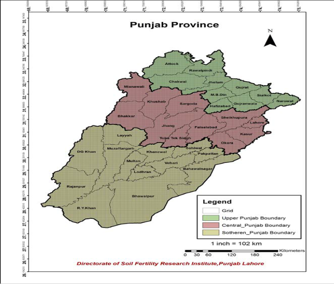
Figure 2.1 Grid Map of Study Area for soil sample location
tial autocorrelation. Two locations with different observations
that up to some extent apart from each other are not statistical
independent.
Generally, geo-statistical estimation methods were exercised to explore and map the agricultural land. It was based on the theory of regionalized variables which were disseminated in space with spatial coordinates and show spatial autocorrela- tion such that samples close together in space are more alike than those that are further apart.

Spatial Dependence

Explores the tendency among the observations that are close together in space consider more correlated/interrelated with each other than those that were at distant. It is also called spa-

Semi- Variance

Describes function of distance between the two observations is a measure of the spatial dependence.

Semi-Variogram

Represents a graph that shows how distance between the ob- servations changes as the semi variance changes. As a function of distance between observations is used to measure the de- gree of dissimilarity is semi-variogram. It is based on “Rule of

IJSER © 2013 http://www.ijser.org

International Journal of Scientific & Engineering Research, Volume 4, Issue 11, November-2013 328

ISSN 2229-5518

Geography” that things close together are more alike than things that are at a distant. Two observations/locations are close to each other, semi- variance generally behaves low. Sim- ilarly, semi- variance increases as the distance between the
Mathematically, semi-variogram is descirbed as a func- tion below:
locations grow until a saturation point comes where these lo- cations are considered independent of each other and semi- variance no longer increases.
The weights in the kriging method are based on the distance between the measured points and the prediction points and

γ ( h ) =

N ( h )

[ z ( x ) − z( x

+ h)]2

the overall spatial arrangement of the measured points. Spatial

2N (h)

∑ i i

i =1

prediction defines optimally by using this method. Mathematically, kriging is described as a function be-
Where N (h) is the total number of data pairs separated by a distance h; Z represents the measured value for soil property, and x is the position of soil samples. Before the geo-statistical estimation, a semi-variogram is calculated for classes of dis- tance between sample pairs. Standard models are used to fit the experimental semi-variogram, e.g., spherical, exponential, gaussian in this study.

Variogram

Method or semi-variogram technique describe the measure of spatial variability of a soil with regionalized variable that pro- vides the input parameter like electrical conductivity (EC), for the spatial interpolation of kriging.
A variogram is generally characterized by three phases.

Nugget

The inconsistency/variability in the field data refers nugget that cannot be described with respect to distance among the observations. Variability of the field data which is being measured and imprecision in sampling techniques influences the magnitude of nugget. The nugget can also be influenced by the minimum distance between the observations, because if they are not located close to each other, then the spatial de- pendence among observations cannot be estimated.

Sill

low:

Where
=Value to be predicated at location
=Observed value at sampling location
n =number of locations within the search neighborhood area used for the prediction [1, 2 and 14]

Criteria for Comparison of Best Fitted Model

In order to find out the best fitted model in ordinary kriging interpolation method, Spherical, Exponential, Gaussian and K- Bessel functions are used in this study. Model selection for semi-variograms is done by comparing the deviation of esti- mated value from the observed/measured data and perform- ing a cross-validation test over the entire dataset. The cross- validation technique is used to choose the best variogram model among candidate models and to select the search radius and lag distance that minimises the kriging variance. The val- ues of mean error (ME), root mean square error (RMSE), Av- erage standard error (ASE), Mean standardized error (MSE) and root mean square standardized error are estimated to check the results/performance of the best fitted theoretical models.
Maximum observed variability/inconsistency in the field data refers sill. The amount of observed variation that can be de-

1

Mean Error =

N

∑[Z(xi ) −

Zˆ ( xi )]

scribed by distance among observations is the main difference between sill and nugget. A small nugget and a large sill would be an ideal situation (i.e., there is a lot spatial dependence and an unpredicted location could be inferred much based on its distance from an observed location).

N i =1

Root Mean Square Error =

1 N

[Z(x ) −

Zˆ ( x )]2

Range

The range is that saturation point at which the semi-variance stops growing. The distance at which two observations are unrelated/dissimilar (i.e., independent) represents range.

∑ i i

i =1

1 N

Interpolation Method

Spatial distribution pattern of soil EC was determined using the geo-statistical technique providing the interpolation meth- ods such as Kriging.

Average Standardized Error =

1

∑σ2 (x )

N i =1

N ME

Kriging

In geo-statistical techniques, Ordinary Kriging is one of the most optimal tools that provide an estimate at an unsampled point based on the weighted average of observed adjacent points within a respective area. It is best linear unbiased esti- mation for quantities which vary in space.


Mean Standardized Error = ∑ 2

Nσi =1(x ) i

IJSER © 2013 http://www.ijser.org

International Journal of Scientific & Engineering Research, Volume 4, Issue 11, November-2013 329

ISSN 2229-5518

1 N ME

the kriging variance for location

Root Mean Square Standardized Error =

∑( )2

i =1 i

Where is the predicted value, the observed
(known) value, N the number of values in the dataset and is
The following rules should be implemented in order to get best fitted model:
• The mean error (ME) should ideally be zero.
• An accurate model would have a mean standardized er-
ror (MSE) close to zero.
• If the model for the variogram is accurate, then the root
mean square error (RMSE) should equal to the average
standard error (ASE).
• Root mean square standardized (RMSP) should equal 1.
• Standard deviation should be greater than Average
standard error (ASE).
If the RMSS is greater than 1, then the variability in the predic-
tions is being underestimated, and vice versa. Similarly if the
average standard errors (ASE) are greater than the root mean
square standardized errors (RMSS), then the variability is
overestimated, and vice versa [ 4, 6, 10 and 11]

Data Analysis

Statistical results indicated that soil EC was fitted for normal logarithmic distribution .GIS software packages were used to analyze different data sets. Maps were developed with GIS software ArcGIS and its extension of Spatial Analyst and Geo- statistical Analyst extention. The geostatistical analysis and the probability calculations were carried out with geostatistic ex- tension of ArcMap.

RESULTS AND DISCUSSION

Tables below summarize EC datasets, which includes descrip- tive statistics such as minimum, maximum, mean, median, mode, standard deviation, skewness and kurtosis. Before per- forming geostatistical analysis, the raw dataset was logarith- mically transformed to make the dataset normally distributed of soil EC.

Table 3.1: Descriptive Statistics of EC (Upper Punjab)

Table 3.2: Descriptive Statistics of EC (Central Punjab)

IJSER © 2013 http://www.ijser.org

International Journal of Scientific & Engineering Research, Volume 4, Issue 11, November-2013 330

ISSN 2229-5518

Table 3.3: Descriptive Statistics of EC (Southern Punjab)

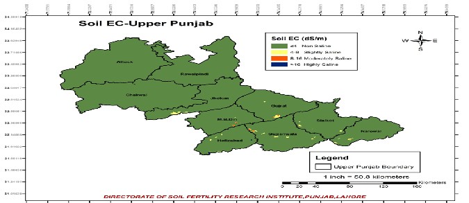
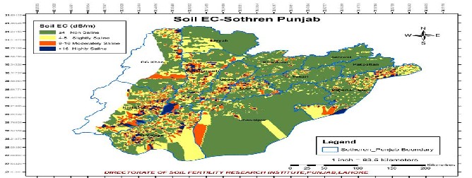
Based on this statistics, the upper Punjab that includes Rawal- pindi & Gujranwala divisions represent average soil EC of about less than 4 (ds/m) or non-saline. In contrast, the south- ern Punjab that includes Multan, DG Khan & Bahawalpur rep- resent high EC zone on the average due to concentration of salt. And central Punjab that includes Sargodha, Faisalabad & Lahore division lied in the category of highly saline in some
tehsils and on the average it was moderately saline.

Log Transformation of Soil-EC

Transformation was done to normalize dataset of soil-EC for three sampled zone of Punjab province, which was proposed as Upper Punjab, Central Punjab and Southern Punjab.

IJSER © 2013 http://www.ijser.org

International Journal of Scientific & Engineering Research, Volume 4, Issue 11, November-2013 331

ISSN 2229-5518

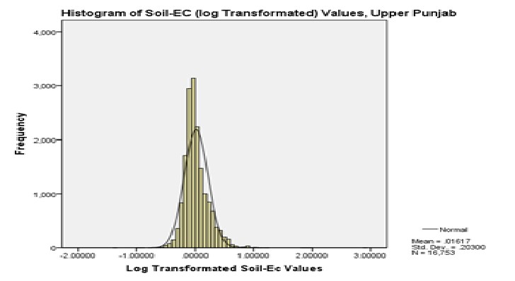
Figure 3.1

IJSER © 2013 http://www.ijser.org

International Journal of Scientific & Engineering Research, Volume 4, Issue 11, November-2013 332

ISSN 2229-5518

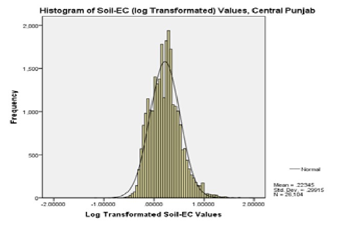
Figure 3.2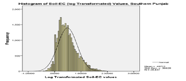

Figure 3.3

IJSER © 2013 http://www.ijser.org

International Journal of Scientific & Engineering Research, Volume 4, Issue 11, November-2013 333

ISSN 2229-5518

Normal distribution in statistics is described by the continuous line of histogram with mean and standard deviation, which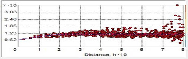

Semi-Variogram

Figure 3.4 Semivariogram for Log-transformated EC values
A semi-variogram of soil EC is shown in figure given below to find out the behavior of spatial dependence of data by using geostatistical wizard, which shows strong spatial dependence
were estimated from the data by applying log transformation.
in right by using spherical model and weak spatial depend- ence in left by using circular model.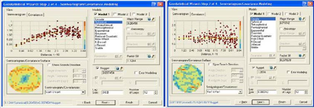

Figure 3.5
EC-Geostatistical analysis results were presented in tables be- low. It showed that to predict Soil EC, Spherical, Gaussian and Exponential models of Kriging method were chosen for its estimation. The highest precision and minimum error were the basic reason for the prediction of soil EC. The models
spherical, exponential and Gaussian has been analyzed and compared with each other to get the optimum results of best fitted model.

Table 3.4: Results of geostatistical analyses of Soil EC in Upper Punjab

IJSER © 2013 http://www.ijser.org

International Journal of Scientific & Engineering Research, Volume 4, Issue 11, November-2013 334

ISSN 2229-5518

Table 3.5: Results of geostatistical analyses of Soil EC in Central Punjab

Table 3.6: Results of geostatistical analyses of Soil EC in Southern Punjab

By performing the cross- validation of Soil EC, the spherical& exponential models were best to choose to estimate the soil EC. To validate the accuracy of interpolation, we implemented the cross validation in soil dataset .During this process, a small subset of actual dataset is removed which consist of a few soil samples. And the predicted value of this subset in its location
is observed with the remaining observation of the actual da- taset. By comparing the measured and predicted results, we also found out the average difference between measured and predicted values as well. These are the cross validation graphs for the dataset used to create the semi-variogram above.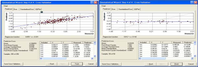

Figure 3.6

IJSER © 2013 http://www.ijser.org

International Journal of Scientific & Engineering Research, Volume 4, Issue 11, November-2013 335

ISSN 2229-5518

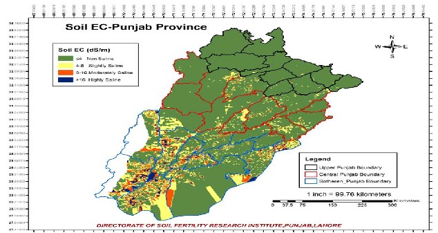
If data is correlated, then get a similar value which is predict- ed at that location by removing sample for cross-validation as shown in right above. But if spatial dependence is weak in dataset, then it is not possible that the predicted value of any removed sample will approximately equal to the arithmetic average value of dataset. In order to find out spatial variation of Soil EC, a predicted map was provided by kriging method for agricultural land of Punjab province. The confined area had different types of soil with respect to EC, Which was mainly defined with respect to some ranges as described
below:
Based on these maps, the upper Punjab that includes Rawal- pindi & Gujranwala divisions represented soil EC of about 8 or slightly saline. In contrast, the southern Punjab that in- cludes Multan, DG Khan & Bahawalpur represented high EC zone. And central Punjab that includes Sargodha, Faisalabad
& Lahore represent EC less than 16 almost which is less than the mean EC in other agricultural land in Punjab province.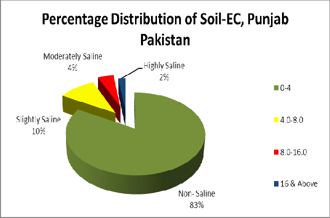

Figure 3.7

IJSER © 2013 http://www.ijser.org

International Journal of Scientific & Engineering Research, Volume 4, Issue 11, November-2013 336

ISSN 2229-5518

According to given study, EC of Soil Punjab represented 83%
area of Punjab were Non-Saline, 10% were slightly saline, re-
maining 4% were Moderately saline and only 2% of agricul- tural land was highly saline.

3.3 Interpolated Map of Soil EC of Upper Punjab

3.4 Interpolated Map of Soil EC of Central Punjab

IJSER © 2013 http://www.ijser.org

International Journal of Scientific & Engineering Research, Volume 4, Issue 11, November-2013 337

ISSN 2229-5518

3.5 Interpolated Map of Soil EC of Southern Punjab

3.6 Interpolated Map of Soil EC of Punjab Province

CONCLUSION

1. Kriging is most suitable method found, other than any interpolation methods and spherical and expo- nential variogram probably is inconsequential.
2. Both behave similarly in terms of predictive accuracy in order to find out spatial variability of EC in agricul-

IJSER © 2013

tural land of Punjab province.
3. Based on the predicted map of soil EC in Punjab
Province, electrical conductivity is found higher in
Southern Punjab than in the Upper and Central Pun-
jab areas.
4. Almost all the agriculture land in southern Punjab is
faced a lot of salinity related problems.
http://www.ijser.org

International Journal of Scientific & Engineering Research, Volume 4, Issue 11, November-2013 338

ISSN 2229-5518

5. The central Punjab represents a moderately saline soil with respect to EC.
6. upper Punjab represents almost a non-saline soil in all
agricultural fields within this area.
7. One of the main challenges in agriculture land of
Punjab province is salinity, its reduction and control.

REFERENCES

[1] Robinson, T. and G. Metternicht. Testing the performance of spatial interpolation techniques for mapping soil properties, Computers and Electronics in Agriculture. 50(2006), 97-108.
[2] Deutsch, C., A. Journel. GSLIB: Geostatistical software library and user’s guide, Oxford University Press, Oxford, UK..
(1998).
[3] Douaik, A., M. Meirvenne and T. Toth. Soil salinity mapping using spatiotemporal kriging Bayesian maximum entropy with interval soft data, Geoderma.128 (2005), 234-248.
[4] Johnston, K., J. M. Ver Hoef, K. Krivoruchko and N.. Lucas. Using ArcGIS Geostatistical Analyst, Environmental Sys-
tems Research, Redlands, USA. (2001).
[5] Kastens, T. and S. Staggenborg. Spatial Interpolation Accuracy, Kansas State Precision Ag Conference, January 29-30,
2002, Great Bend, Kansas.(2002)
[6] Kravchenko, A. and D. Bullock. A comparative study of interpolation methods for mapping soil properties, Journal of
Agronomy, 91(1999), 393–400.
[7] Mohamed, M. and B. Abdo. Spatial variability mapping of some soil properties in El-Multagha agricultural project
(Sudan) using geographic information systems (GIS) techniques, Ministry of Agriculture and Forestry, Sudan.(2011). [8] Nawar, S., R. Mohamed, F. Farag and A. Nahry. Mapping Soil Salinity in El-Tina Plain in Egypt Using Geostatistical
Approach, Fac. of Agric. Suez Canal Univ., Egypt.(2011).
[9] Poshtmasari, H., Z. Sarvestani, B. Kamkar, S. Shataei and S. Sadeghi. Comparison of interpolation methods for estimat- ing PH and EC in agricultural fields of Golestan province (north of Iran), International Journal of Agriculture and Crop Sciences, IJACS. 4-4 (2012), 157-167.
[10] Voltz, M. and R. Webster. A comparison of kriging, cubic splines and classification for predicting soil properties from sample information, Journal of Soil Sciences. 41(1990), 473–490.
[11] Webster, R. and M. Oliver. Geostatistics for Environmental Scientists, John Wiley and Sons, Brisbane, Australia.
[12] Wilson, R. Freeland, R. Wilkerson, J. and Hart, W. (2005). Interpolation and data collection error sources for Electromag- netic induction-soil electrical Conductivity mapping, American Society of Agricultural Engineers ISSN 0883−8542.
21(2001).
[13] Zandi, S., A. Ghobakhlou and P. Sallis. A Comparison of Spatial Interpolation Methods for Mapping Soil pH by Depths, Geo-informatics Research Centre, Auckland University of Technology New Zealand.(2011).
[14] Zhang, C. and D. McGrath. Geostatistical and GIS analysis on soil organic carbon concentrations in grassland of south-
eastern Ireland from two different periods, Geoderma. 119(2004), 261-275.

IJSER © 2013 http://www.ijser.org