International Journal of Scientific & Engineering Research, Volume 4, Issue 11, November-2013 207
ISSN 2229-5518
Real-time Traffic Congestion Detection using
Combined SVM
Sukriti Sharma, Vidya Meenakshi.K, Apurva VS, Saritha Chakrasali, Shreyas Satish.
Abstract— Traffic density and flow are important inputs for an intelligent transport system (ITS) to better manage traffic congestion. This paper proposes a cost effective traffic congestion detection system by using image processing algorithms and a combined Support Vector Machine (SVM) classifier and thereby demonstrates the efficiency of using key informative metrics like edge and texture features in real time. Effectiveness of the proposed method of classifying traffic density states is demonstrated on real time traffic images taken at different time periods of a day in Bangalore city.
Index Terms— Virtual loop detector (VLD), Traffic density, SVM Classifier, ITS, Feature extraction, Image processing, Combined classifier
—————————— ——————————
eavy traffic congestion poses a big problem in almost all capital cities around the world, especially in developing regions resulting in massive delays, increased fuel waste
and monetary losses..To reduce traffic congestion, various traffic management techniques are being developed continu- ously. ITS being one among them uses advanced applications which aims to provide innovative services relating to different modes of transport and traffic management thus enabling var- ious users to be better informed and make safer, more coordi- nated, and 'smarter' use of transport networks. Traffic density is required by the ITS to operate other higher level functionali- ties such as sequencing traffic lights and organizing control signals. The Loop Detector (LD) is one of the most widely ap- plied techniques in detecting the traffic density. The paper by Luigi DI Stefano et al., “Evaluation of Inductive-Loop Emula- tion Algorithm for UTC Systems” uses LD. A loop detector is installed close to an intersection point and triggers some sig- nals once a vehicle passes over the LD. The accumulated out- put signals from an LD estimates the traffic flow passing in the area where the LD is installed. However, an LD has limitations due to its difficulties in installation and maintaining [1].
To overcome the problem of LD, the paper by Zhidong Li et al., “On Traffic Density Estimation with a Boosted SVM Classi- fier “ aimed to develop a Virtual Loop Detector (VLD) that simulates a real LD by using a machine learning approach to detect the traffic density in real-time. The paper proposes a boosted SVM classifier with some informative features to dis- tinguish between a zero-occupancy (ZO) state and a non-zero- occupancy (NZO) state. Here, the traffic density is defined as the occupancy of vehicles on a road surface [1]. The outputs from the VLD are used to detect the traffic density at a given Region of Interest (ROI). However, the complexity of combin- ing the results of individual SVMs is higher.
In this paper SVM classifiers are used to classify the traffic density into a high or low state. Instead of Adaboost [1], the complexity has been reduced by applying the product rule on the results of individual SVMs. Only critical texture and edge features such as energy, uniformity etc. are selected. There- fore, the sizes of the feature vectors are reduced, optimizing feature extraction.
This paper uses image processing algorithms for feature ex-
traction that can be used to analyze CCTV camera feeds from traffic cameras which will further help the SVM to detect and classify traffic congestion levels into low density or high den- sity in real time. If in a continuous flow of images, a majority of the images is classified as high density, a traffic congestion warning is sent to the respective authority.
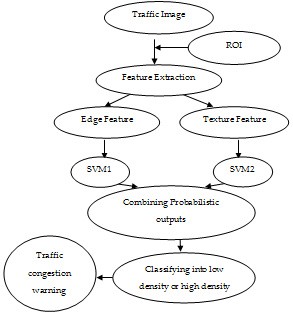
System flow of the proposed algorithm is shown in Fig.1, which comprises of feature extraction, SVM training, and real- time traffic congestion detection as three main components. An ROI area is manually defined to indicate the coverage re- gion of a VLD across the images [1]. The traffic density classi- fication is in terms of low and high density of traffic.
Fig. 1 System flow of the proposed algorithm
IJSER © 2013 http://www.ijser.org
International Journal of Scientific & Engineering Research, Volume 4, Issue 11, November-2013 208
ISSN 2229-5518
Used in both pattern recognition and image processing, fea- ture extraction is a special form of dimensionality reduction. Transforming the input data into the set of features is called feature extraction. If the features extracted are carefully chosen it is expected that the features set will extract the relevant in- formation from the input data in order to perform the desired task using this reduced representation instead of the full size input.
Features are efficient in distinguishing between the traffic density states in this system. Enhanced texture and edge fea- tures are used as they are efficient in distinguishing the traffic density states and are not too sensitive to illumination changes [13]. The gray scale image is the input for the proposed algo- rithm. Further ROI selection is the preprocessing applied to the input image.
Edges are significant local changes of intensity in an image. Edges typically occur on the boundary between two different regions in an image. Edge features are supposed to reflect the fact that more vehicles on the road would result in more edges in the image. In this paper, an Edge Orientation Histogram algorithm is applied to the ROI area [14].
To extract edge features, the basic idea is to build a histogram with the directions of the gradients of the edges (borders or contours). The gradient is the change in gray level with direc- tion. This can be calculated by taking the difference in value of neighboring pixels. The detection of the angles is possible through Sobel Operators. The next five operators could give an idea of the strength of the gradient in five particular direc- tions (Fig.2).
Fig. 2 The Sobel masks for 5 orientations: (a): vertical, (b): horizontal, (c)
and (d): diagonals, (e): non-directional
The input to the Edge Orientation Histogram algorithm is the source image which consists of the path to the ROI. The out- put is a vector with 5 dimensions representing the strength of the gradient in the five directions – horizontal, vertical, diago- nals, non-directional. We first calculate the size of the image in terms of width and height and build a matrix with the same size and 5 dimensions to save the gradients for each direction. The filter for each direction is applied to the source image and the result is stored in the matrix created. The maximum gradi- ent is obtained from the matrix and the type of the gradient is used to build the histogram. To eliminate redundant gradi- ents, canny edge detection is applied to the source image. The type of maximum gradient is multiplied with the resulting image after applying edge detection. To build the histogram, the image is divided into clips and the histogram is built for each clip with 5 bins [14]. Then, the values of the histogram for each clip are averaged over each direction to obtain a final vector of 5 dimensions.
Considering vehicles as the 'grains' in the texture, more cars residing in the Region of Interest brings a coarser texture while fewer or no vehicles would have a closer texture distri- bution to the road surface itself [1].
In this paper, the method adopted by Zhidong Li et al is ap- plied to calculate the texture statistics [1].
Firstly, the ROI input image is scaled into 16 gray levels. Secondly, the first order statistics are calculated. First order measures are statistics calculated from original image values and do not consider the pixel neighborhood relationships.
Let L be the number of distinct gray levels and z be the ran- dom variable denoting the gray-levels, then p (zi ), (where i=0,
1,...L-1), is the probability of a gray level occurring in an im- age. To calculate the probability of occurrence of intensities, first a histogram of intensity is built with 16 levels each repre- senting a gray level. Then, the length for each gray level is divided with total number of pixels to obtain the probability of its occurrence.
We then calculate the 5 dimensions used for 1st order statistics. The dimensions are: Mean, Overall Standard deviation (SD), R-Inverse variance (IV), Overall uniformity, Overall Entropy. Thirdly, the second order statistics are calculated-
To calculate the second order statistics, the positional opera- tors used are: 0°, 90°, 45°, 135° with a distance of 1 unit. The symmetric GLCM and its corresponding statistical descriptors are calculated for each image with each positional operator. It’s descriptors are then averaged over the four angles to give a rotationally-invariant texture feature description.
Let cij be a normalized element of a GLCM where i is the row position and j is the column position. The texture descriptors
used are: Angular Second moment (ASM), Dissimilarity, En- ergy, Contrast, and Correlation.
Each image is represented by two separate feature vectors consisting of texture and edge features respectively.
V = [ t1 t2 t3 t4 t5 t6 t7 ] E = [e1 e2 e3 e4 e5]
In the texture vector V, ti (where i=1, 2, 3…7) represents the texture feature dimension. Only selected features are consid- ered for the vector as explained in Chapter 5. t1 represents Inverse variance, t2- Uniformity, t3- Entropy, t4- ASM, t5- Dis- similarity, t6- Energy, and t7- Correlation. In the edge vector E, ej (where j=1, 2...5) represents the edge feature dimension. e1 to e5 represents the number of pixels with increasing intensity in the direction of maximum gradient, where e5 represents the number of pixels of maximum intensity in the direction of maximum gradient.
SVM is mainly used for classification. In the training phase, the input fed to the SVM is the feature vector extracted from the images. In this work, two SVM classifiers are trained with the edge feature vectors and texture feature vectors extracted from the sample training images respectively. After fitting the model, the feature vectors extracted from sample testing im-
IJSER © 2013 http://www.ijser.org
International Journal of Scientific & Engineering Research, Volume 4, Issue 11, November-2013 209
ISSN 2229-5518
ages are fed into the respective SVM. The output is in terms of probability of the test image belonging to each class, low den- sity and high density. The proposed algorithm aims at com- bining the results of the SVM on edge feature vector and SVM on the texture feature vector to improve the efficiency, using product rule. Product rule is an effective method to combine classifiers trained with different image descriptors. When the classifiers have small errors and operate in independent fea- ture spaces, it is very difficult to combine their (probabilistic) outputs by multiplying them. Thus, this product rule is used to determine the final decision. First the posterior probability outputs Pj k (xk) for class j of n different classifiers is combined with the product rule as shown in (1).
tains both day time and night time images. Different ap- proaches evaluated in this paper include an SVM with the tex- ture feature, an SVM with the edge feature and combining both texture and edge features using product rule. The train- ing data covers day time and night time images and similarly the testing is evaluated on the images covering both day and night images. Fig. 4, Fig. 5 shows some sample preprocessed training images used. Fig. 6 shows a few preprocessed testing samples used.
n
P (x1 ....x n ) = π P
(x k )
(1)
j k =1 j
Where xk is the pattern representation of the kth descriptor. Then the class with the largest probability product is consid- ered as the final class label belonging to the input pattern [16].
Fig. 3 Flow diagram of combined classifier
This work uses traffic images taken from the cameras installed at various junctions by the Bangalore Traffic Police. This con-
H1 H2 H3 H4
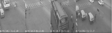
Fig. 4 Sample preprocessed training images-High density at day
L1 L2 L3 L4
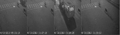
NL1 NL2 NL3 NL4
Fig. 5 Sample preprocessed training images- Low density at day: Low1-5, Low density at night: NLow1-4

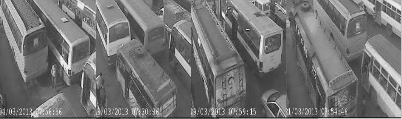
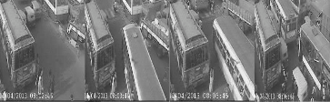
Test1 Test2 Test3 Test4
IJSER © 2013 http://www.ijser.org
International Journal of Scientific & Engineering Research, Volume 4, Issue 11, November-2013 210
ISSN 2229-5518
![]()
Test5 Test6 Test7 Test8
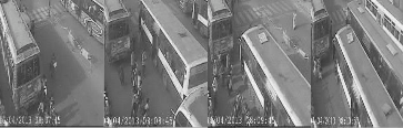
Test9 Test10 Test11 Test12
Fig. 6 Sample preprocessed testing images
The edge results obtained after applying edge histogram de- scriptor is given in Table 1, which gives the strength of the gra- dient. It shows the number of pixels with varying intensity in the direction of maximum gradient. Here, E1 is the number of pixels with minimum intensity; E5 is the number of pixels with maximum intensity in the direction of maximum gradient. It is observed that the value for number of pixels of maximum in- tensity in the direction of maximum gradient have increased for high density, i.e., E5 have increased for high density in day time because there are more number of edges in that direction.
The texture results shown in Table 2 reflect that for images with low density of traffic, the pixel distribution will be closer to the road surface. As it is seen in Table 2, the values for ASM, Energy(Eng.), Uniformity (Unf.), IV increase for images with low density of traffic.
Since for images with high density of traffic, there is more var- iation around the mean, and more difference in gray levels, the values for dissimilarity(Diss.), entropy(Ent.) increase for those images. As it is seen in Table 3, there is no significant trend in the variations of values for mean and standard devia- tion(SD). Hence, it has been decided to remove those features from the texture vector as they may create problems for the SVM to classify accurately. Also, after extracting texture vec- tors for more images, it was found that the values for contrast do not show a significant trend. Hence, this feature has not been considered in the final texture vector used for training. TABLE 1 RESULTING FEATURE VALUES AFTER APPLYING EDGE ORI-
ENTATION HISTOGRAM
TABLE 2 RESULTING TEXTURE FEATURE VALUES
TABLE 3 RESULTING DISCARDED TEXTURE FEATURE VALUES
Images | Contrast | Mean | SD |
IJSER © 2013 http://www.ijser.org
International Journal of Scientific & Engineering Research, Volume 4, Issue 11, November-2013 211
ISSN 2229-5518
L1 | 1.01 | 109 | 41.71 |
L2 | 1.18 | 117 | 53.26 |
L3 | 1.20 | 77 | 35.07 |
L4 | 1.12 | 82 | 36.19 |
NL1 | 0.96 | 61 | 31.2 |
NL2 | 0.89 | 62 | 31.4 |
NL3 | 1.29 | 67 | 32.7 |
NL4 | 0.92 | 64 | 31.9 |
H1 | 2.21 | 259 | 64.19 |
H2 | 1.89 | 88 | 37.48 |
H3 | 2.37 | 98 | 39.55 |
H4 | 1.72 | 112 | 42.28 |
![]()
We have trained the SVMs with around 430 images which in- clude day and night images. Table 4 shows the results of tex- ture SVM and edge SVM for 12 sample test images. The results are classified into probability of low density, probability of high density for texture SVM and edge SVM .The cross marks “×” indicates wrongly predicted results. Texture SVM has 4 wrongly predicted results, edge has 3 wrongly predicted re- sults .From the results in Table 4, it is observed that edge SVM is more efficient in distinguishing the traffic density states as it gives less incorrect predictions in comparison with texture SVM.
Table 5 shows the results of the combined classifier that is combination of texture SVM and edge SVM. Here cross mark “×” indicates the wrongly predicted results. It is observed that after combining the individual SVM outputs the number of incorrect predictions has decreased. Texture SVM has 4 incor- rect predictions, edge SVM has 3 incorrect predictions but combined Classifier has only 2 incorrect predictions. Thus the combined classifier has improved the classification accuracy.
TABLE 5 RESULTS OF COMBINED CLASSIFIER
TABLE 4 RESULTS OF TEXTURE SVM AND EDGE SVM
This work proposes a method for traffic density estimation using image processing and machine learning.Images are tak-
IJSER © 2013 http://www.ijser.org
International Journal of Scientific & Engineering Research, Volume 4, Issue 11, November-2013 212
ISSN 2229-5518
en from the live camera feed.The preprocessing done on these images converts them into gray scale versions and identifies the ROI.The ROI is used for further processing.
From the values obtained in Table 1,it is obsereved that the values for the number of pixels of maximum intensity in the direction of maximum gradient have increased for high densi- ty,where the gradient refers to the change in gray level with direction.
From Table 2 it is observed that features like Dissimilarity,
Correlation, Entropy have increased for high density, whereas features for ASM, Energy, IV, Uniformity values have in- creased for low density.The reasons for which were discussed earlier.After obtaining the featuresfor edge and texture, fea- ture vectors were constructed.
As seen in Table 4 It is observed that the edge SVM shows slightly more efficiency than texture SVM.
From the results in Table 5 it is observed that number of incor-
rect predictions have decreased compare to individual SVM
and an overall efficiency of 95% is obtained.
In this work, 5 cosecutive images with a time gap of 1 minute are passed. These images are classified as low or high density and based on value a congestion alert is provided to respective authorities.As 5 images are passed, the threshold value is set as 3.If 3 or more images shows high density, then the final result shows traffic congestion.The results match our expecta- tion.This work can be extended to further junction of Banga- lore city and future enchacement can be provided to remove shadows.
This work is supported by the B.N.M Institute of Technolo- gy,Bangalore and Mapunity Information Services(p) Ltd. Ma- punity works closely with the Bangalore Traffic police and was responsible for helping establish India’s first comprehen- sive traffic management system. It was this system that pro- vided the required data for our project.
[1] L.Zhidong et al., “On Traffic Density Estimation with a Boosted SVM Classifier,” IEEE Trans. Digital Image Computing: Technology and Ap- plocations, Dec 2008, doi: 10.1109/dicta.2008.30.
[2] S.Shiliang, Z.Changshui,Y. Guoqiang,”A Bayesian Network Ap- proach to Traffic Flow Forecasting,” IEEE Trans. Intelligent Transporta- tion Systems, vol.7, no.1, March 2006, doi: 10.1109/ITTS.2006.869623.
[3] G.Surendra et al. (2002),” Detection and Classification of Vehicals,” IEEE Trans. Intelligent Transportation Systems, vol.3, no.1, March 2002, doi: 10.1109/6979.994794.
[4] C.Rita, P.Massimo, M.Paola,”Image analysis and rule-based reason- ing for a traffic monitoring system,” IEEE Trans. ITS, vol.1, no.2, June
2000, doi: 10.1109/6979.880963.
[5] W.Jingbin et al.,”Detection Objects of Variables Shape Structure with Hidden State Shape Models,” IEEE Trans. Pattern analysis and Machine Intelligence, vol.30, no.3, March 2008, doi: 10.1109/TPAMI.2007.1178.
[6] F.Vittorio Ferrari et al., “Groups of Adjacent Contour Segments for
Object Detection,” IEEE Trans. Pattern analysis and Machine Intelligence, vol.30, no.1, Jan 2008, doi: 10.1109/TPAMI.2007.1144.
[7] S.W.Chee, K.P.Dong, J.P. Soo.,” Efficient use of Edge Histogram De- scriptor,” ETRI Journal, 24(1), Feb 2002.
[8] T.Evan, C.Jing,” Vehicular Traffic Density Estimation via Statistical
Method with Automated State Learning,” Proc. IEEE Symp. Adavced
Video and Signal based Surveillance (AVSS2007), pp.164-167, 5-7, Sept
2007, doi: 10.1109/AVSS.2007.4425304.
[9] L.Xiaokun and M.P.Fatih,” A Hidden Markov Model Framework for Traf- fic Event Detection using Video Features,” ICIP, March 2004.
[10] W.Lei, X.Ping, L.C.Kap,” Incorporating Prior Knowledge into SVM
for Image Retrieval,” proceedings of the 17th International Conference on
Pattern Recognition 2004 (ICPR 2004), August 2004.
[11] Z.Shile, F.Jianping, L. Hong,”Salient Object Detection on Large-Scale Video Data,” Proc. IEEE Symp. Computer Vision and Pattern Recogni- tion, pp. 1-6, June 2007, doi: 10.1109/CVPR.2007.383495.
[12] A Berengolts, M. Lindenbaum, “On the Distribution of Salience,” IEEE Trans. Pattern Analysis and Machine Intelligence, vol.28, issue 12, pp 1973-1990, Dec 2006, doi: 10.1109/TPAMI.2006.249.007.
[13] C. G. Rafael and H. W Richard, 2002, Digital Image Processing, Pren-
tice Hall, pp.34-134.
[14] U. Roberto. (2012) “Edge Orientation Histograms in Global and Local
Features,”Jan 26, 2012. Available at: http://roberto.blogs.cultureplex.ca/
2012/01/26/edge-orientation-histograms-in-global-and-local- features/ Feb 13, 2013.
[15] S.Scholkopf et al., 1999, Advances in Kernel methods: Support Vector
Learning, MIT Press, Cambridge.
[16] A.Azizi, C. V .Remco, A. W. Marco, “An Ensemble of Deep Support Vec- tor Machines for Image Categorization, Soft Computingand Pattern Recog- nition,” SOCPAR’09, International Conference, DEC 2009.
Vidya Meenakshi K completed her B.E in information science from BNM Institute of Technology, Bangalore, affiliated to VTU, India in July 2013. Her final year group project titled “ Traffic Density Estimation using SVM Clas- sifier” won best project award in computing division at JED-I national project challenge held at IISC, Bangalore June 2013.
Email: vidya.meena09@gmail.com
Shreyas Satish has been a software engineer for the past three years at Ma- punity - a social technology lab in Bangalore - where he was responsible for building the entire technology stack for Technagara (http://technagara.in) (untilJuly,2013). He received his 'Bachelor of Engineering' in Information Science from the Visvesvaraya Technological University (Belgaum).E- mail:Shreyas.satish@gmail.com.
Saritha Chakrasali is an associate professor at BNM Institute of Technolo- gy in the ISE department. Her research interests are image processing, infor- mation technology, cryptography and network security, intelligent agents. She has published in 5 international conferences and 2 national conferences. She is an organizing committee member for the fifth International conference on signal and image processing (ICSIP 2014).
E-mail:Saritha.chakrasali@gmail.com
IJSER © 2013 http://www.ijser.org