International Journal of Scientific & Engineering Research, Volume 2, Issue 11, November-2011 1
ISSN 2229-5518
Real-Time Sky Color with Effect of Sun’s Position
Hoshang Kolivand, Mohd Shahrizal Sunar
Abstract— In the rendering of outdoor scenes in virtual environments, the sun's position, sky color, clouds, shadow, trees, grass etc play very important roles in making it realistic. In this paper Sky color and the sun’s position are combined. Specific longitude, latitude, date and time are required parameters to calculate the exact position of the sun. The sun's position is calculated based on Julian dating; the sky’s color is created by Perez modeling. A functional application is designed to show the position of the sun and then sky color i n arbitrary location, date and time. It can be possible to use this application in commercial games for outdoor rendering and for teachers to teach some part of physics about earth orbit and effect of the sun on the sky and it can be used in building design.
Index Terms— Sky color, Sun’s position, Real-time, Outdoor rendering
—————————— ——————————
n the rendering of outdoor scenes in virtual environments, the sun's position, sky color, clouds, shadow, trees, grass etc play important roles in making it appear realistic. The prin- ciple calculations of the sun's positions have been very well known for a long time. The ancient Egyptians were able many years ago to calculate the sun's position so. By digging a large hole inside one of the pyramids, just once a year, on the king’s birthday, the sun could shine on the grave of their king [1]. The sun's position and the amount of sunshine have, histori- cally, been a very attractive subject for most of researchers. For example, in 1958, Giover J. et al. worked on the principle amount of sunshine in a day. In 1990, Kambezidis et al. [2] provided several functions to calculate the sun's position by focusing on factors such as light refraction and right ascen- sion. Many ideas and principle concepts can be found in Sayigh et al., published in 1997, Duffie et al. in 1980, Kreider et al. in 1981, Wieder in 1982, Iqbal. in 1983 and Muir in 1983 [3]. Numerous computer graphics researchers have tried to si- mulate the atmospheric effect on the sky. Many of them have simulated the light from the sky and the sun by considering the scattering and absorption of light in the earth's atmos- phere. Early work in rendering and modeling the atmospheric effects was done, in 1982, by Blinn and Max in1986 [4]. Blinn propose a method of modeling Saturn's rings by using thin layers of clouds and dusty surface while Max introduced a single scattering model for light diffusion to generate haze in the atmosphere. In 1987, Klassen [5] tried to display sky color by taking into account spectral distribution due to particles in the atmosphere. However, this method has problems because the atmosphere is approximated as multiple layers of the plane-parallel atmosphere. But it is assume as uniform densi- ty. Thus, the method is different from the actual physical phe- nomenon. In 1991, Kaneda et al. [6] improved this method by approximating the actual physical phenomenon. He consi-
————————————————
Mohd Shahrisal Sunar is currently head of computer graphics department of Universiti Teknologi Malaysia, MALAYSIA, , E-mail
:shah@fsksm.utm.my
dered the spherical atmosphere with air density changing ex- ponentially with altitude. This work had been extended using multiple scattering by Nishita et al. in 1996[7]. Most of the proposed methods can display a realistic sky color but have a time constraint in rendering. Tadamura et al. [8] combined both Kaneda's model and the CIE. They discussed the rela- tionship between them and published their discussion in 1993.
Dobashi et al. in1997 [9], proposed a fast display method of sky color using basis functions. In the proposed method, co- sine functions are used as basis function. The color of sky in the view direction of an arbitrary the sun position can be ob- tained from stored distributions and displayed quickly. The method is tested for natural scenes and architectural design. The problem with this method is not achieving the photo rea- listic target.
In1999, Preetham et al. [10] approached an analytic model for rendering the sky. The image generated is impressive. They present an inexpensive analytic sky model from Perez et al. [11] (Perez model) that approximates full spectrum day- light for various atmospheric conditions. At the same time, they also presented a model for aerial perspective, which en- hanced the realism of outdoor rendering.
Sunar et al. [12] in 2001 created a sky dome simulate the ef-
fect of the sun's position on sky color using the Perez model.
In 2007, Sheng Li et al [13] proposed unified volumes repre-
sentation for light shaft and shadow, which is an efficient me-
thod of simulating natural light shafts and shadows with at-
mospheric scattering effect. In 2008, Halawani et al. [14] tried to produce illuminated 3D objects based upon the effects of
interaction between the sunlight and sky and Sunkavalli et al. [15] proposed a model for temporal color changes and ex- plores its use for the analysis of outdoor scenes from time- lapse video data.
The most important effect of the sun's position is on sky color. The position of the sun depends on location, date and time. Location depends on longitude and latitude but the effect is different on different days of the year.
Latitude is a distance from north to south of the equator. Lon- gitude is the angular distance from east to west of the prime meridian of the Earth. Longitude is 180 degrees from east to
IJSER © 2011
International Journal of Scientific & Engineering Research, Volume 2, Issue 11, November-2011 2
ISSN 2229-5518
west. Each 15 degrees represents one hour of time. For exam- ple, if you were to travel west at 15 degrees per hour, you would, one hour later, have travelled for an hour with no change in the actual time. The earth spins around the sun in specific orbit once year.
The angle between earth's orbit and the equator is 23.5 degrees at all times because the angle that the sun can be seen is differ- ent at different latitudes. Sunset and sunrise are produced by rotation of the earth. The first place that can see sunrise in each day is Japan [16]. This is the main reason that there are differ- ent days of the month, different seasonal months and different seasons of the year.
These ranges are used to create a specific part of the dome because in sky modeling, the north part of the sky dome is all that is needed.
Knowing zenith and azimuth are enough to calculate the position of the sun. To have zenith and azimuth, location, lon- gitude, latitude, date and time are needed. Zenith is the angle that indicates the amount of sunrise while the azimuth is the angle that indicates the amount angle that the sun turns around the earth.
In 1983, Iqbal [17] proposed a formula to calculate the sun's position and in 1999, Preetham et al. [10] improved it. It is a
Before determining the sun's position, the sky must be
modeled. To create the sky, virtual dome is a convenient tool.
There are two ways to model the dome; using 3D modeling
t ts 0.17 sin(
SM L
4 ( j 80)
![]()
373
) 0.129 sin(
![]()
2 ( j 8) )
355
software such as 3D Max or Maya and using a mathematical
function. Mathematical modeling is adopted for this real-time environment.
A dome is like a hemisphere in which the view point is lo- cated inside. To create a hemisphere using mathematical for- mulas the best formula to use is:![]()
12
common formula to calculate the position of the sun in phys- ics.
where
t: Solar time
x2 y 2
z 2
r 2
(1)
ts: Standard time
The above formula in angular system is
Where is the zenith and is the azimuth and
f ( ,) cos2 cos2 sin 2 cos2 sin 2 r 2
J: Julian date
SM: Standard meridian
L: Longitude
The solar declination is calculated as the following formula:![]()
0.4093sin 2 ( j 81)
368
: Solar declination
The time is calculated in decimal hours and degrees in ra-
dians.
Finally zenith and azimuth can be calculated as follows: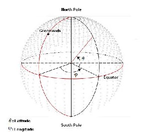
![]()
cos sin t
tan1 ( 12 )
s
![]()
cos l sin sin l cos cos t
12
![]()
![]()
sin 1 (sin l sin cos l cos cos t )
s 2 12
Fig 1: The zenithal and azimuthal angles on the hemisphere
Where is the zenith and is the azimuth and
Where![]()
: Solar zenith
: Solar azimuth
L: Latitude
With calculation of zenith (![]() )and azimuth (
)and azimuth (![]() )the sun's posi-
)the sun's posi-
tion is obvious. To have the sun’s position a Cartesian coordi-
nate is needed. The point (x, y, and z) is the position of the sun
and it is specific in every location, date and time.![]()
0
2
0 2
IJSER © 2011
International Journal of Scientific & Engineering Research, Volume 2, Issue 11, November-2011 3
ISSN 2229-5518
Traditionally, colors have been described in words, usually by allusion to common objects such as "red apple", "green spi- nach" or "blue sky". More precisely, color is communicated in the painting and dying industry by production of charts of sample colors. The numerical specification of color has a long history that began with the famous physics legend, Sir Isaac Newton. It was only in the twentieth century that numerical systems became important in industry.
The interaction of light, an object and the eye creates color. There must be a light to illuminate the object. As said in Poyn- ton, color is the perceptual result in the visible region of the spectrum, having wavelengths in the region of 400 nm to 700 nm, incident upon the retina. The human retina has three kinds of color preceptor cone cells with peak sensitivities to
580 nm ("red"), 545 nm ("green") and 440 nm ("blue"). This is stated in the tri-stimulus theory of color perception in Apple (1996).
In 1931, The Commission International De l'Eclairage (CIE) [18] developed a device-independent color model that was based on human perception. It is known as the CIE XYZ mod- el that defines three primaries known as X, Y and Z. The three primaries can be combined to match with any color that hu- mans see which is related to the tri-stimulus theory of color perception. The topic of CIE color spaces will be discussed in more detail in the color spaces section.
Although there are approximately four billion colors that humans can see, color is normally divided into eleven basic categories. As Berlin and Kay said in 1969 [19], the eleven ba- sic categories are white, black, red, green, yellow, blue, brown, purple, pink, orange and grey.
The color perceived by our eyes is not the pure color of the object. The color had been scattered on its journey to our eye. Therefore, the color of the tree at the mountain is not the same as the tree in front of our eyes.
In computer graphics and old commercial games, the color of the sky was blue but sky color is not simply blue. During the course of a day, the color of the sky changes with the posi- tion of the sun. The sky color around the horizon and zenith is different almost all the time. When color of sky is blue, near the horizon it is close to white. At the start or at the end of the day, or at sunrise and sunset, the color of the sky becomes red, orange and white. The most important cause of these various colors is the scattering of aerosols and air molecules. Sky color is related to the suns direction, date, time and location of viewpoints. To calculate the sky color, several methods are proposed but all of them consider just single scattering. Multi scattering can produce high quality sky color for virtual envi- ronments [20].
The scattering of incoming sunlight is very important for the brightness and color of sunlight and skylight. Scattering is the process by which small particles suspended in a medium of a different index of refraction diffuse a portion of the inci-
dent radiation in all directions. Figure 2 illustrates scattered sunlight in atmospheric articles. Oxygen and nitrogen are two examples of air molecules, which are small in size. Thus, they are more effective at scattering shorter wavelengths of light (blue and violet). The selective scattering by air molecules is responsible for producing our blue skies on a clear sunny day. Most of the atmospheric particles can be assumed to be spher- ical and homogeneous. For this reason, Rayleigh and Mie scat- tering theories can be used to describe the scattering. In 1881, Lord Rayleigh [21] introduced a scattering theory for the scat- tering of light by the molecules of the air. It can be extended to the scattering of particles of up to about a tenth of the wave- length of the light. The scattering theory is known as Rayleigh scattering.
Mie scattering theory involves scattering particle sizes larg-
er than a wavelength. The theory is suitable for particles of a diameter from at least twice the wavelength of the light source. Gustav Mie presented the Mie scattering theory in
1906 [22].
To represent color information in terms of intensity values, a color space is modeled. The dimensions or components that represent intensity values are defined in 1D, 2D, 3D or 4D spaces. Each component of color is also referred to as a color channel.
There are several different color spaces available. This will give the appropriate working with whichever type of color data is best. It can be categories as grey spaces, RGB, CMYK, device-independent color spaces, named color spaces and he- terogeneous HiFi color spaces.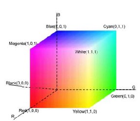
Fig 2: The RGB color space
The XYZ space allows the color to be expressed as a mix- ture of the three tri-stimulus values X, Y and Z. The CIE stan- dard allows a color to be classified as a numeric triple (X, Y, Z). All the CIE-based color spaces are derived from the fun- damental XYZ space.
IJSER © 2011
International Journal of Scientific & Engineering Research, Volume 2, Issue 11, November-2011 4
ISSN 2229-5518
CIE XYZ space accepts all colors perceivable by human be- ings and it is based on experimentally determined color matching functions. Thus, it is a device-independent color space.
All visible light can be shown as a positive combination of
X, Y and Z. Therefore, Y component almost associates to the
apparent lightness of a color. In general, the mixture of X, Y
and Z components that describe a color can be expressed as
percentages.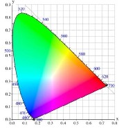
Fig 3: CIE color space for xy chromaticity’s.
Yxy space is another space that determines the XYZ values in terms of x and y chromaticity co-ordinates. To convert XYZ space into Yxy co-ordinates the following formulas are used:
Y Y
the behavior of the particular phosphor in a specific monitor. For that reason, creating a general transformation matrix to obtain an accurate color conversion is not possible. Sometimes a CIE XYZ value will give a negative value when converted to a RGB color space, but RGB values cannot be any negative. The negative value is out of the RGB gamut that defines no color. Therefore, a color matching process is needed. Hence, some colors that are described in the CIE color space cannot be described in the RGB color space.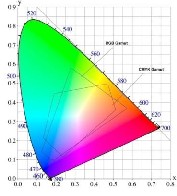
Fig 4: Color Gamut for two devices expressed Yxy
The Perez model is convenient method to illuminate arbi- trary point of the sky dome respect to the sun's position. The Perez model uses CIE standard and it can be used for a wide range of atmosphere with different conditions. Luminance of point can be calculated by using the following formula:![]()
x X
X Y Z
![]()
y Y
X Y Z
L(
p ,
B
![]()
) (1 Ae cos p )(1 CeD p E cos 2 )
For the other way around, to convert from Yxy co-ordinates
cos1 (sin
sin p
cos( p
s ) coss
cos p )
to XYZ, the following formulas can be used:![]()
X x Y
y
Y Y
Z 1 x y
Where
A: Darkening or brightening of the horizon
B: Luminance gradient near the horizon
C: Relative intensity of circumsolar region![]()
y Y D: Width of the circumsolar region
E: Relative backscattered light received at the earth surface
The Z tri-stimulus value is not visible by itself and is com- bined with the new co-ordinates. The layout of color in the x and y plane of Yxy space is shown in Figure 4. This diagram is well known as the wing-shaped CIE chromaticity diagram, which is extensively used in color science.
In another situation, to convert between the device inde- pendence CIE based color space to a device dependent RGB color space in computer graphics, a color transformation ma- trix is essential. It is useful for mapping the CIE XYZ values to RGB monitor values. Nevertheless, this conversion is not easy. It is because the trans- formation matrix is dependent upon
The zenith values and skylight distribution coefficient are specified in Preetham et al., 1999 [10]. The calculation can be shown by the matrices below. The values of zenith are the functions of turbidity (T) and the sun’s position, while a dif- ferent T value will give a different distribution coefficient.
Distribution coefficients for luminance, Y distribution func- tion:
IJSER © 2011
International Journal of Scientific & Engineering Research, Volume 2, Issue 11, November-2011 5
ISSN 2229-5518
AY
not only in terms of the sun angle and intensity of radiation, which are different every time, but it is affected by changes in
B
0.1787
1.4630
the color of light and contrast. At dawn, when the sun is not
Y
0.3554
0.4275
T
yet over the horizon, the sky along the horizon will be golden
C 0.0227
5.3251
shiny and bright purple. When the sun can be seen over the
Y
1
D
Y
E
0.1206
0.0670
2.5771
0.3703
horizon, the sky becomes yellow and then an attractive blue
color.
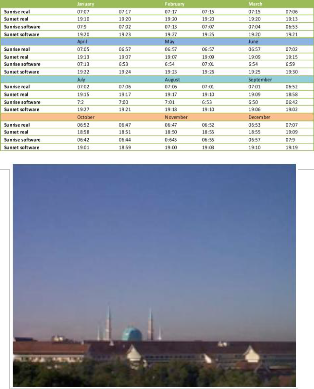
The results Table 1 show the real and application generated
Y
A
data for sunrise and sunset in the first day and last day of each month in Universiti Teknologi Malaysia at latitude of 1.28 and
x
0.0193
0.2592
longitude of 103.45 at different times of the day.
B
T
x
0.0665
0.0008
1
Cx 0.0004
0.2125
TABLE 1. THE REAL AND APPLICATION GENERATED DATA FOR SU-
D
0.0641
0.8989
NRISE AND SUNSET TIME OF UNIVERSITI TEKNOLOGI MALAYSIA
x
0.0033
0.0452
Ex
Ay
B
y
0.0167
0.0950
0.2608
0.0092
C 0.0079
0.2102
T
y
0.0441
1.6537
1
Dy
y
0.0109
0.0529
Absolute value of zenith luminance:
4
T 2 ![]()
Yz=(4.0453T-4.9710)tan
9![]()
120
s -0.2155T+2.4192
Zenith x, xz and zenith y, yz are given by following matrix:
3
1.00166
0.00375
0.00209
0 s
2
x T 2
T 1 0.02903
0.06377
0.03202
0.00394 s
s
0.11693
0.21196
0.06052
0.25886
1
3
0.00275
0.00610
0.00317
0 s
2
y T 2
T 1 0.04214
0.08970
0.04153
0.00516 s
Fig 5: Real sky’s color (UTM, 15 June, 2011)
0.15346
0.26756
0.06670
0.26688 s
1
Sky color and the sun's position in real-time computer games can make a game as realistic as possible. To keep the real position of the sun in a virtual environment, a substantial amount of precision is needed. Solar energy is free and a bless- ing from God, but optimized usage of this blessing needs a mastermind. On the other hand, in building design and archi- tecture, possible recognition of which direction is best to build a building in specific location.
For a period of one year, the amount of sunshine in the southern hemisphere is more than the northern hemisphere except for latitude less than1.5 degree. The sky’s color changes with the position of the sun during the day and even at night. In nature, image quality varies every minute. The changes are
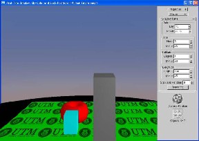
Fig 6: Result of application (UTM, 15 June, 2011)
IJSER © 2011
International Journal of Scientific & Engineering Research, Volume 2, Issue 11, November-2011 6
ISSN 2229-5518
The sky color as determined by the sun’s position, are the most important factors to consider when creating realistic outdoor scenes. The main target of this study was to develop a daylight sky’s color with effect of sun’s position. Thus, four objectives were determined in order to achieve the goal. First, the dome sky, which was modeled using mathematical func- tions, is a better way to represent the sky. The algorithm not only supports a triangular mesh, but also a quadratic mesh. The sun’s position needs to be calculated by Juliann dating. Finally the color of the sky had to be carried out using Perez modeling which yields the result in CIE Yxy space.
A model that gives the sky’s color according to the sun’s position and the specific location, date and time has been de- veloped. A software package of the real-time sky’s color with effect of sun’s position simulator was successfully constructed in C++ OpenGL. All the objectives were met in order to reach the main goal.
There are some extensions that can be made to this project. It is possible that the software could model not only the sky but also other natural phenomena such as cloud, landscape and the ocean. Shadow is another natural phenomenon that can make this package more complete and more realistic.
This research was supported by UTMVicubeLab at Depart- ment of Computer Graphics and Multimedia, Faculty of Com- puter Science and Information System, Universiti Teknologi Malaysia. Special thanks to Universiti Teknologi Malaysia (UTM) Vot. 00J44 Research University Grant Scheme (RUGS) for providing financial support of this research.
[1] S. Nawar, A.B. Morcos, J.S. Mikhail,” Photoelectric study of the sky brightness along Sun’s meridian during the March 29,” New Astron- omy, Vol. 12, pp. 562–568,2007.
[2] H.D. Kambezidis, D.N. Asimakopoulos, C.G. Helmis, ”Wake Mea- surements Behind a Horizontal-Axis 50 kW Wind Turbine, ” Solar Wind Tech Vol. 7, pp. 177-184,1990.
[3] M.S. Sunar, M.N. Zamri,” Advances in Computer Graphics and
Virtual Environment” UTM Malaysia, 2007.
[4] J.F. Blinn, ”Light refection functions for simulation of clouds and dusty surfaces,” ACM Transactions on Graphics, Vol. 16:21-29, 1982.
[5] R.V. Klassen,” Modeling the effect of the atmosphere on light, ” ACM
Transactions on Graphics, Vol. 6, pp. 215-237, 1987.
[6] K. Kaneda, T. Okamoto, E. Nakamae, T. Nishita, ” Photorealistic image synthesis for outdoor scenery under various atmospheric con- ditions, ” The Visual Computer, Vol. 7, pp. 247-258, 1991.
[7] T Nishita, E. Nakamae, Y Dobashi, ” Display of clouds and snow taking into account multiple anisotropic scattering and sky light, ” In Rushmeier, H., ed., SIGGRAPH 96 Conference Proceedings, Annual Conference Series, 379-386. Addison Wesley. held in New Orleans, Louisiana, 04-09 August 1996.
[8] K. Tadamura, E. Nakamae, K. Kaneda, M. Baba, H. Yamashita, T.
Nishita,” Modeling of Skylight and Rendering of Outdoor Scenes, ”
Computer Graphics Forum, Vol. 12, pp. 189-200, 1993.
[9] Y. Dobashi, T. Nishita, K. Kaneda, H. Yamashita,” A fast display method of sky colour using basis functions,” The Journal of Visuali- zation and Computer Animation, Vol. 8, pp. 115-127, 1997.
[10] A.J. Preetham, P Shirley, B. Smith, ” A practical analytic model for
daylight,” Computer Graphics,(SIGGRAPH '99 Proceedings), 91-100,
1999.
[11] R. Perez, R. Seals, J. Michalsky, ”All-weather model for sky lumin- ance distribution - preliminary configuration and validation,” Solar Energy, Vol. 50, pp. 235-245, 1993.
[12] M.S. Sunar, N.A. Gordon,”Real-Time Daylight Sky Color Modeling,”
Advances in Computer Graphics and Virtual Environment, 37-55,
2001.
[13] S. Li, G. Wang, E. Wu, ”Unified Volumes for Light Shaft and Shadow
with Scattering,” IEEE, 161-166, 2007.
[14] S.M. Halawani, M.S. Sunar,” Interaction between sunlight and the sky color with 3D objects in the outdoor virtual environment,” Fourth International Conference on Mathematic/Analytical Model- ing and Computer Simulation, 470-475, 2010.
[15] V.M. Viswanatha, Nagaraj B. Patil, M.B. Sanjay Pande, Processing of Images Based on Segmentation Models for Extracting Textured Component, International Journal of Scientific & Engineering Re- search Vo. 2, no. 4, April-2011.
[16] D. Gutierrez, F.J. Seron, A. Munoz, O. Anson, ” Simulation of at-
mospheric phenomena,” Computers & Graphics, Vol. 30, pp. 994-
1010 , 2006.
[17] M. Iqbal, ”An introduction to solar radiation,” Academic Press. 1983, pp. 390.
[18] CIE, International commission on illumination. http://www.cie.co.at/cie/home.html,2011. Cited 16 July 2011.
[19] B. Berlin, P. Kay, ” Basic color terms,” Berkeley: University of Cali- fornia, Reprinted, 1991.
[20] B.W. Kimmel, G.V.G. Baranoski, ”Simulating the appearance of sandy landscapes,” Computers & Graphics, Vol. 34, pp. 441-448,
2010.
[21] L. Rayleigh,” Experiments on colour,” Nature (London), 25, pp. 64–
66, 1881.
[22] R Penndorf, MIE scattering in the forward area. Infrared Physics, Vol. 2, pp. 85-102, 1962.
IJSER © 2011