To highlight this, suppose the vehicle is excited with a 2 2
sine-wave input x(t) of amplitude A and frequency f in
hertz, then:
International Journal of Scientific & Engineering Research, Volume 5, Issue 2, February-2014 795
ISSN 2229-5518
Quadrotor Comprehensive Identification from
Frequency Responses
Abubakar Surajo Imam, Robert Bicker
Abstract— Design and development of a quadrotor model-based flight control system entails the use of the vehicle's dynamic model. It is quite challenging to use the physical laws and first principle-based approaches to model the quadrotor dynamics as they are highly nonlinear, characterized by coupled rotor-airframe interaction. However, system identification modeling method provides a less challenging approach to modeling the dynamics of highly non-linear systems such as a quadrotor. This paper presents the frequency-domain system identification procedure for the extraction of linear models that correspond to the hover flight operating conditions of a quadrotor. Frequency response identification is a versatile procedure for rapidly and efficiently extracting accurate dynamic models of aerial vehicles from the measured response to control inputs. During the extraction of the quadrotor's model, flight test manoeuvres were used to excite the variables of concern for flight dynamics and control by adopting a systematic selection procedure of the model structure for the parameterized transfer-function model and the state-space model. The technique provides models that best characterized the vehicle's measured responses to the controls commands, and can be used in the design of a flight control system.
Index Terms— Dynamic model, flight control system, frequency-domain system identification, flight dynamic and control, excitation and measured responses, quadrotor.
—————————— ——————————
Recently, the use of small-scale rotorcraft unmanned aerial vehicles (UAVs) for surveillance and monitoring tasks is be- coming attractive. Amongst the various configurations of the small-scale rotorcraft, the use of a quadrotor gained more prominence, particularly in the research community [1], [2], [3], [4], [5]. A quadrotor is a small responsive four-rotor vehi- cle controlled by the rotational speed of its rotors. It is com- pact in design with the ability to carry a high payload.
The dynamics of rotorcraft is substantially more complex than that of a fixed-wing aircraft [6], the complexity increases as the vehicle become smaller. The high non-linear nature of a quadrotor makes difficult the use of physical law and first principle-based approach to model its dynamics. The quad- rotor dynamics is characterized by the coupled rotor-airframe dynamics. Hence, system identification method is needed to model the dynamics of non-linear systems such as a quad- rotor, and the procedure is conducted in either time or fre- quency domain. A number of studies have reported the use of system identification procedure to identify the dynamics of rotorcraft [7], [8], [9], [10]. For instance, a method for system identification using Neural Networks was proposed in [7], where input-output data was provided from nonlinear simula- tion of X-Cell 60 small-scale helicopter, and the data was used to train the multi-layer perceptron combined with NNARXM time regression input vector to learn nonlinear behavior of the vehicle. A rotorcraft system response data was acquired in carefully devised experiment procedure in [8], and a time do- main system identification method was applied in extracting a linear time-invariant system model. The acquired model was used to design a feedback controller consisting of inner-loop attitude feedback controller, mid-loop velocity feedback con- troller and outer-loop position controller, when implemented on the Berkeley RUAV, the controllers showed remarkable hovering performance. Similarly, parametric and non- parametric models for a rotorcraft were identified using data
collected through identification method in [10], after which two control laws were designed for the vehicle attitude stabili- zation. In [11], system identification method was applied to examine a high-bandwidth rotorcraft flight control system design. In the study, flight test and modeling requirements were illustrated using flight test data from a BO-105 hingeless rotor helicopter. A systematic way is adopted in this study to derive a quadrotor dynamics models using the frequency- domain system identification method. Once the models are determined, a single-input-single-output (SISO) and multiple- input-multiple-output (MIMO) control loops can be designed and implemented on a quadrotor
System identification is the procedure for deriving a mathematical model of a system based on experimental data of the system’s control inputs and measured outputs. The procedure involves derivation of a mathematical mod- el based on experimental data of the vehicle's control in- puts and measured outputs; it also provides an excellent tool for improving mathematical models used for rotorcraft flight control system design. System identification method can be used for derivation of both parametric and nonpar- ametric models: examples of nonparametric models in- clude impulse and frequency response models, and exam- ples of parametric models are transfer function and state space models. The nonparametric models are directly de- rived using experimental data and provide an input– output (I/O) description of the system. These model types are based on collections of data and do not require any knowledge of the system structure. However, the challenge
IJSER © 2014 http://www.ijser.org
International Journal of Scientific & Engineering Research, Volume 5, Issue 2, February-2014 796
ISSN 2229-5518
of the system identification procedure is to derive a para- metric model of a system. The first step towards the extrac- tion of a parametric model is the derivation of a parameter- ized model, which will serve as a logical guess of the actual system model. The use of an optimization algorithm de- termines the parameters of the model that minimize the error between the actual system responses and the model responses. Estimates of those characteristics may be ob- tained by analysis of the nonparametric model combined with information obtained by the first principles approach. The system identification procedure is an iterative process. Depending on the identification results, the parameterized model may be refined in terms of order and structure until a satisfactory identification error is achieved. When the parameterized model is known, the system identification method reduces to the parameter estimation problem [12]. A Key application of rotorcraft system identification results include piloted simulation models, comparison of wind
control inputs. Flight test manoeuvres are used to excite the variables of concern for flight dynamics and control, or struc- tural stability. Typical excitations used in system identification are frequency sweeps and doublets. The techniques provide a model that best characterizes the vehicle's measured responses to controls commands [15], such as (i) frequency response model, (ii) transfer function model and (iii) state space model.
This is a nonparametric model which represents the out- put/input amplitude ratio and phase shift of a system in an effective format, such as a Bode plot. It can be regarded as a data curve identified from the flight test data, which represent the ratio of the response per unit of control input as a function of control input frequency. The frequency response is obtained using the fast Fourier transform and associated windowing techniques.
This model provides a closed-form equation that is a good representation of a frequency response data. The model is of the form:
tunnel test versus flight measurements, validation and im-
(b s m + b s m−1 + ...... + b
)e−τs
provement of physic based simulation models, flight con-
T(s)
= 0 1 m
s n _ a s n−1 + ..... + a
(1)
trol system development and validation 1 n
There are numerous methodologies for system identifica- tion techniques which are well described in [13], [14]. A major classification amongst these methodologies depends on whether the compared responses are considered in the time or frequency domain. The similarities between fre- quency-domain and time-domain methods are; in both, good results depend on proper excitation of key dynamic modes; multiple inputs should not be fully correlated; both can be used for parametric model identification that can be verified in the time domain. The major differences between the two are; the initial data for frequency-domain method
The values of the numerator coefficients (b 0 , b 1 , ... bm )
and denominator coefficients (a1 .....an) are determined us- ing system identification procedure. The transfer function is a parametric model comprising a limited set of character- istics parameters.
This can is the parametric model of the complete differential equation of motion that describes the MIMO behaviour of the vehicle. Equation (2) represents the linear differential equation for a small perturbation about a trim flight condition in state- spac. e.
consists of frequency responses derived from time-history
x = Ax + Bu(t − τ )
(2)
data, while the time-domain method initial data consists of time history data. In addition, time domain method pro- vides both linear and nonlinear models, whereas frequency domain method provides only a linearized characterization of the system, and a describing function for a nonlinear model. There exist none independent metrics to assess sys-
Where the control vector u is composed of the control inputs and the vector of the vehicle states x comprises the response quantities (speed, angular rates, and attitudes angles). The
time-delay vector τ allows for a separate time-delay value for
each control. However, the set of available flight-test meas-
urement y is composed of a subset of the states and given by:
tem excitation and linearity in time-domain method,
whilst, in frequency-domain method there are a number of
y = Cx + Du(t − τ )
(3)
metrics such as coherence function, Cramer-Rao inequality and cost function.
System identification as applied to a quadrotor is a versa- tile procedure for rapidly and efficiently extracting accurate dynamic models of rotorcraft from the measured response to
The values of the matrices A, B, C, D and the vector τ are
determined using the system identifications procedure.
Based on [12] and [15] frequency domain identification is an ideal way for extracting linear rotorcraft models of high accuracy. One of the main advantages of this approach is
IJSER © 2014 http://www.ijser.org
International Journal of Scientific & Engineering Research, Volume 5, Issue 2, February-2014 797
ISSN 2229-5518
the use of actual flight data for deriving and validating the model. Additionally, frequency domain identification has a coherent flow of the design steps starting from the input– output characterization of the vehicle (nonparametric mod- eling), continuing with the extraction of the state space model (parametric modeling) concluding with validating the predicted model in the time domain. This method is classified as an output-error method where the fitting error is defined between the actual flight data frequency re- sponses and the frequency responses predicted by the model.
In the frequency response system identification technique, the following independent metrics are used to measure model accuracy in terms of system excitation, data quality and sys- tem response linearity:
The products of the Fourier transform computation are the Fourier coefficients of the input X(f) excitation and output Y(f) response. This leads to the definition of the three spectral func- tions (i) input spectrum, (ii) output spectrum and (iii) cross spectrum. Based on [17], a rough estimate of the input auto- spectrum is determined from the Fourier coefficients by:
![]()
![]()
![]()
To highlight this, suppose the vehicle is excited with a 2 2
sine-wave input x(t) of amplitude A and frequency f in
hertz, then:
G xx ( f ) =
T
X ( f )
(8)
x(t ) = A sin(2πft )
When the transient response has decayed, the system output
(4)
Similarly, a rough estimate of the output auto-spectrum or input PSD displays the distribution of the output squared or response power as function of frequency given by:
y(t) will also be a sine wave of the same frequency f, but with an associated amplitude B and a phase shift ϕ :![]()
G yy
![]()
![]()
( f ) = 2 Y ( f ) 2
T
(9)
y(t ) = B sin(2πft + ϕ )
(5)
Finally, a rough estimated of the cross spectrum or cross PSD
displays the distribution of the product of input multiplied by
This implies that for a linear time-invariant (LTI) system,
a constant sine-wave periodic input results in a constant sine-wave output at the same frequency f, referred to as the
output or input-output power transfer as a function of fre- quency, and is given by:
first harmonic frequency. It is therefore important to note, for linear systems, the higher harmonics of the response are not considered, as the time function is the same for the in-![]()
G yy
![]()
![]()
![]()
![]()
( f ) = 2 Y ( f ) * Y ( f )
T
(10)
put and output. For these systems, the focus is on the am- plitude A and B, phase shift ϕ . The parameter values A, B and ϕ in this case, can be obtained from the time-history
plots or calculated numerically using the Fourier series for only the first harmonic terms [16].
The frequency response function H(f) is a complex-
Note that, the cross spectrum is a complex-valued function
and thus conveys input=output phase information.
The coherence function is an important product of the smooth spectral functions. It can be interpreted as the fraction of the output spectrum that is linearly attributable to the input spec- trum at a certain frequency.
valued function defined by the data curves for the magnifi- cation and phase shift at each frequency f given by:
2
G xy ( f )
γ 2 ( f ) =
(11)
![]()
![]()
![]()
H ( f ) = B( f )
A( f )
![]()
![]()
< H ( f ) = Phase Shift = ϕ ( f )
(6)
(7)
G xx ( f ) G yy ( f )
The coherence function is a normalized metric having a value ranging from zero to unity. It is an indicator of the linearity between the input and output. A value of the coherence func- tion close to unity indicates that the output is significantly linearly correlated with the input of the system. In practical
The frequency response can be obtained experimentally by exciting the system with discrete sine-wave inputs.
applications, there are several reasons for a low value of the coherence function [18]. Following a simple guide, the coher- ence function can be used to effectively and rapidly examine the accuracy of frequency-response identification [12]. Gener-
IJSER © 2014 http://www.ijser.org
International Journal of Scientific & Engineering Research, Volume 5, Issue 2, February-2014 798
ISSN 2229-5518
ally, if the coherence function satisfies Equation (12), and is not oscillating, then the frequency response can be said to have acceptable accuracy [15].
tablishes the nonparametric model of the vehicle. The design of the parameterized linear state space model follows using information from the physical laws and the nonparametric modeling phase.
γ 2 ≥ 0.6
(12)
The Cramer-Rao inequality is another reliable measure of pa- rameter accuracy in the frequency-response identification method. The inequality establishes the Cramer-Rao bounds (CR) as the minimum expected standard deviation in a pa- rameter estimate obtained from many repeated manoeuvres. The Cramer-Rao bound is given by:
σ ≥ CR
(13)
Relative values of the Cramer-Rao bounds associated with the identification parameters are of key significance for refining the model structure. High values of Cramer-Rao bounds for individual parameter suggest indicate poorly identified pa- rameters and suggest these parameters to be removed or fixed in the model structure.
The quadratic factor J referred to as cost function is also useful in deciding an acceptable level of model accuracy. For flight dynamic modeling, a cost function of J ≤ 100, generally repre- sents an acceptable level of accuracy, whereas a cost function of J ≤ 50 is expected to produce an exact match of the flight data.
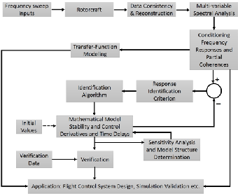
Fig. 1 illustrates the sequence of a frequency response identifi- cation procedure, in which the initial step is the excitation of the vehicle using specially designed input signals, such as a frequency sweep, to excite the vehicle dynamics over a desired frequency range. The choice of the desired frequency range has an important role in the identification process and has to be wide enough in order to capture all the dynamic effects of interest (i.e., airframe and rotor dynamics).
After some preprocessing to eliminate the noise and other types of inconsistencies in the time domain output data, the second phase computes the input–output frequency responses using a Fast Fourier Transform. This phase of the process es- tablishes the nonparametric model of the vehicle. The design of the parameterized linear state space model follows using information from the physical laws and the nonparametric modeling phase.
After some preprocessing to eliminate the noise and other types of inconsistencies in the time domain output data, the second phase computes the input–output frequency responses using a Fast Fourier Transform. This phase of the process es-
Fig. 1. Flowchat for frequency response system identification.
After some preprocessing to eliminate the noise and other types of inconsistencies in the time domain output data, the second phase computes the input–output frequency responses using a Fast Fourier Transform. This phase of the process es- tablishes the nonparametric model of the vehicle. The design of the parameterized linear state space model follows using information from the physical laws and the nonparametric modeling phase.
The frequency domain identification method is only suitable for the derivation of a linear parametric model. Although the rotorcraft dynamics are nonlinear, around certain trimmed flight conditions, the nonlinearities from the equations of mo- tion and aerodynamics are relatively mild. When this is the case, a linearized model is sufficient to accurately predict the vehicle's response. Usually, the validity of the linearized mod- el is adequate over a wide area of the flight envelope around the trim point. However, a single linear model in most cases is not sufficient to represent globally the flight envelope. There- fore, different models are required for each operating condi- tion. The final step of the identification procedure is the vali- dation of the model. This step takes place in the time domain, with different flight data from the identification procedure. For the same input sequence, the vehicle responses from the flight data are compared with the predicted values of the model, obtained by integration of the state space model. How- ever, if the validation portion of the problem is not satisfactory the parametric modeling setup should be modified and the procedure repeated.
A number of software packages can be used for rotorcraft frequency-response identification. Amongst the popular
IJSER © 2014 http://www.ijser.org
International Journal of Scientific & Engineering Research, Volume 5, Issue 2, February-2014 799
ISSN 2229-5518
ones include: MATLAB/SIMULINK, NI Labview and CIFER (Comprehensive Identification from Frequency Re- sponses). MATLAB and LabView are generalized packages which for solving various engineering problems. However, CIFER© software package was developed at Ames research centre primarily for the task of aircraft and rotorcraft fre- quency response identification from flight-test data, and hence it is well suited for application in this study. The program is composed of six utility packages that interact with a sophisticated database of frequency responses. The importance of a well organized and flexible database sys- tem is very crucial in a large scale MIMO identification procedure of an air vehicle. The CIFER© package is de- signed to cover all the intermediate steps necessary for the development of air vehicles parametric modeling. The key characteristic of CIFER© is its ability to generate and ana- lyse high quality frequency responses for MIMO systems, by using Discrete Fourier Transform (DFT) and windowing algorithms [19].
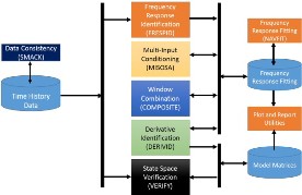
The CIFER® software facilitates the use of frequency domain analysis of flight data to achieve a number of objectives, in- cluding handling quality analysis and specification compli- ance, vibration analysis, and identification of linearized mod- els. The package contains various utilities that can be used interactively as shown in Fig. 2.
Fig. 2. CIFERs software and database components.
Fig. 2 depicts how the CIFER software package is linked to a relational database utility to facilitate the computation of the frequency response identification method of Fig. 3.
The six core programs within the CIFER perform the following processes: data conditioning and performing FFTs, FRESPID; multi-input conditioning, MISOSA; window combination, COMPOSITE; transfer-function model identification, NAVFIT; state-space model identification, DERIVID and model verifica- tion, VERIFY. The package also has utilities that allow inter- facing to many standard data formats, including MATLAB, Excel, ASCII comma and tab delimited, among others. Fre- quency responses generated during any session of the system
identification procedure are stored and catalogued in a dedi- cated database folder. The database entry that is available to all CIFER programs and utilities contains all the information about how the procedure was carried out. In addition, the da- tabase can be shared by multiple users of CIFER and multiple databases can be combined or compressed.
Fig. 3. CIFER software components.
As depicted in Fig 3, time-history data enters the system at two points. The first set of time-history is processed into fre- quency responses at the beginning of the CIFER procedure. At the end of the procedure, a second set of time-history data from inputs dissimilar from those used for the identification is then used for the model verification.
Three programs are run sequentially to generate the MIMO frequency-response database. Beginning with the time-history data, FREPID computes SISO frequency response for a range of spectral windows using a chirp z-transform. The results are then written into the frequency-response database. Next, MISOSA reads in the SISO data from the frequency-response database and conditions these responses for the effect of mul- tiple, partially correlated controls that might have been pre- sent in the same manoeuvre record. Again, the results are written back to the database. Finally, COMPOSITE performs optimization across the multiple spectral windows to achieve a final frequency-response database with excellent resolution, broad bandwidth and low random error.
Two programs support parametric model identification. NAVFIT is used to identify a pole-zero transfer-function mod- el that best fits a selected SISO frequency-response. DERIVID is used to identify a complete generic state-space model struc- ture that best fits the MIMO frequency-response database. Lastly, VERIFY is used to check the identified model's time- domain response based on time-history data from manoeuvres different from those used for the identification.
An important utility program is the smoothing from aircraft
IJSER © 2014 http://www.ijser.org
International Journal of Scientific & Engineering Research, Volume 5, Issue 2, February-2014 800
ISSN 2229-5518
kinematics (SMACK), although not part of CIFER software package, is used for processing of time-history data before the identification proper. Table 1 summarizes the functions of the CIFER components.
Table 1
Summary of the CIFER components functions
Serial | Component | Function |
1 | Time history data | Input to FRESPID and SMACK |
2 | SMACK | Data consistency |
3 | FRESPID | Frequency-response identification |
4 | MISOSA | Multi-input conditioning |
5 | COMPOSITE | Window combination |
6 | NAVFIT | Transfer-function identification |
7 | DERIVID | State-space model identification |
8 | VERIFY | State-space model verification |
This section presents the general requirements and procedure that leads to the comprehensive frequency response system iden- tification of a quadrotor using the CIFER software package. The description of the vehicle platform used has been presented in [25].
An important and challenging aspect in parametric model identification process is the proper selection of the different aspects of model structure that depends on many factors, criti- cal amongst include (i) the ultimate application of the model; (ii) selection of the input-to-output variable pair; (iii) selection
lenge here is deciding on which stability derivatives should be included in the development of the parameterized model. To sim- plify the identification task, the linear parameterized model used for parameter identification of the quadrotor is based on Mettler’s model (with some modifications) described in [20], [21], [22] for the Carnegie Mellon’s Yamaha R-50 and MIT’s X-Cell-60. The
structure of the parameterized model proposed by Mettler has
already been successfully used for the parametric identification of several helicopters of different sizes and specifications [23] and [24]. The ability of this model structure to establish a generic solution to the small-scale rotorcraft identification problem is based on two important factors: a) that the Mettler’s parameter- ized model provides a physically meaningful representation of the system dynamics. All stability derivatives included in this model are related to kinematic and aerodynamic effects of the airframe and the rotor systems, and b) the ability to represent the many cross-coupling effects that dominate the rotorcraft motion. This allows for the integration of the rotors model with the linear- ized equations of motion. The modifications made to the pro- posed parameterized model is due to the absence of a stabilizer bar on quadrotor, which provides additional damping to the pitch and roll rates. However, this function on the quadrotor is ad- dressed by proportional regulation of the rotor speeds.
The quadrotor physical model structure represents direct im- plementation of the equations of motion of the vehicle. In a sys- tem identification procedure, the choice of model structure de- pends on those points highlighted previously. Hence, Equations (2) and (3) can be written in the state-space form as:
.
of frequency range of the fit; (iv) selection of the order of nu-
merator (n) and denominator (m); (v) inclusion of the equiva- lent time delay τ and (vi) fixing or freeing specific coefficients
in the fitting process.
M x = Fx + Gu(t − τ )
.
y = H 0 x + H1 x
(14)
(15)
A transfer-function model is the linear input-to-output description of a dynamic system; it represents the simplest form of paramet- ric model that can be extracted from the numerical frequency- response database. The transfer-function model is sufficient for describing the majority of the quadrotor dynamics, including handling quality analysis, rotors and airframe models and flight control system design. In transfer-function modeling, the system to be modeled is treated like a black box with no attempt to rep- resent the actual dynamics of the vehicle. Transfer-function mod- els are composed of a numerator and denominator polynomial in the Laplace variable s, with an equivalent time delay to account
The matrices M, F, G and vector τ contain model parameters
to be identified as well as the known model parameters and con- stants. Time delays are sometimes included to account for un- modeled system dynamics. A measurement vector y is included to account for the difficulty associated with directly measuring the state x. The matrices H0 and H1 are composed of known con- stants, such as gravity, unit conversion, kinematics, etc. However, once the identification parameters are determined, Equations (14) and (15) can easily be expressed in the conventional state-space- form (Equations 2 and 3):
for additional unmodeled high frequency dynamics and transport delays in the system. However, despite this simplification, the transfer-function model can provide a remarkably accurate repre-
A = M −1F
B = M −1G
(16) (17)
sentation of system response behaviour and has the form of Equa-
tion (1). The order of the numerator and denominator orders are
C = H 0
+ H M −1 F
(18)
selected in such that a good fit of the frequency-response data in the frequency range of interest is achieved.
D = H M −1G
(19)
Determination of the parameterized model is one of the critical aspects in the frequency domain identification method. The chal-
There are nine states and four control variables in the quadrotor's
6-DOF equations describing its airframe motion, centre of mass
IJSER © 2014 http://www.ijser.org
International Journal of Scientific & Engineering Research, Volume 5, Issue 2, February-2014 801
ISSN 2229-5518
(CM) and body rotation, given by:
u2 u3
u1 u4
x = [u
u = [u1
v w
u2 u3
p q r φ
u ]T
θ ψ ]T
(20)
(21)
0 0 0 0
0 0 0 0
0 0
B = Yu
2
Y Y Y
3 1 4
(24)
Where vB = [u, v, w]
and ω =[p, q, r]T
denote the linear and
L L 0 0
2 3
angular velocities components of the vehicle relative to the body-
N N
L Y
u 2
u3 u1
u4
fixed frame.
0 0
L L
During the vehicle's take-off, the output vector consists of the
0 0
N 1 4
quadrotor's linear and angular velocities, and aZ , the linear accel- eration along z-axis. However, at hover flight, acceleration along the x and y axes equals zero, and the vector is reduced to:
T
The unknown coefficient to be identified in matrices A and B
of the parameterized model structure are the conventional
stability and control derivatives, which result from Taylor-
series representation of the vehicle's aerodynamics, composed
of stability and control derivatives of the vehicle, and are a
y = [u v w
p q r
az ]
(22)
complex combination of the vehicle geometric parameters, aerodynamic parameters and inertia parameters. These deriv- atives also represent the complex combination of the quad-
The quadrotor parameterized state-space model represents the linearized dynamics of the perturbed states and control inputs of the helicopter from a trimmed reference flight condition. The trim operating condition considered is the hover mode. Although the parameterized model is associated with the per- turbed values of the states and inputs, the linear state-space parameterized model is given by:
rotor geometric and inertial parameters.
The identification procedure for the quadrotor starts with the collection of the experimental time domain flight data. For each flight data record, the quadrotor was set to hover, and a piloted frequency sweep excitation signal was applied to the four-control variables (u1 , u2 , u3 , u4) one after the other. The bandwidth of the
0
0
0
0
A = 0
0
L
0 − g
0 0
0 0
0 0
0 0
0 0
0 0
0 0 0 0
0 0 0 0
0 0 0 0
0 0 0 Nθ
0 0 0 0
0 0 0 0
0 0 0 Y
0 0
0
0 0
0
Nφ 0
0 Nψ
0 0
(23)
excitation signal ranges between 0.2 – 20 rad/sec, whilst the fre-
quency sweep was executed by the primary input of interest, the secondary inputs were kept uncorrelated to the main input main- taining the vehicle near the reference operating point. For each control input, four records have been collected; the minimum and maximum frequency of the excitation sweeps and the duration of the flight records for each control input are shown in Table 2.
θ θ
Table 2
0 Lφ 0
0 0 Lψ
0 0 0 0
0 0 0 0
Yφ 0
0 ψ
![]()
![]()
Summary of the CIFER components functions
![]()
The variables collected for the identification process were the Euler angles θ, ϕ, ψ; angular velocities p, q, r and body frame acceleration aZ as well as the linear velocity w. For translation, the body frame accelerations were selected instead of the velocity measurements, as these provide a more symmetrical response around the trim value, facilitating the calculations of the respec- tive FFTs. After the collection of the time domain experimental
IJSER © 2014 http://www.ijser.org
International Journal of Scientific & Engineering Research, Volume 5, Issue 2, February-2014 802
ISSN 2229-5518
data, flight records excited by the same primary control input were concatenated into a single record. The time domain experi- mental data was then entered in the CIFER software and pro- cessed using the PRESPID, MISOSA and COMPOSITE to pro- duce a high quality MIMO frequency response database. This database comprises the conditioned frequency responses and par- tial coherences for each input–output pair.
After calculating the flight data frequency responses, the par- ametric models were extracted using the NAVFIT module to de- termine the model transfer-function parameters. The DERIVID module was used to extract and determine the state-space model and its parameters. In both cases, the model parameters were de- termined such that the estimated frequency responses provide best fits to the flight data frequency responses.
The first task executed in the parametric modeling process was the determination of the flight data frequency response input- output pairs, to be included in the identification process, followed by the determination of the frequency range of interest. For the quadrotor, the selected frequency responses and their correspond- ing ranges are depicted in Table 5.9. The coherence function ϒ2 has been used as the criterion for the frequency response selec- tion, for which the coherence function has values greater than 0.6 over the desired frequency range of the model.
The determination of the frequency response pairs to be in- cluded in the identification process was followed by extraction of the transfer-function model; which involved determining the structure and order of the parameterized model, and followed by making initial guesses for the values of the model parameters. CIFER uses an optimization algorithm which computes the cost function J satisfying Equation 5.20 for each input-output pair. The optimization algorithm is based on an iterative robust secant algorithm that reduces the phase and magnitude error between the state space model and the flight data frequency responses. The execution of the optimization algorithm continues until the aver- age of the selected frequency responses and cost functions are minimized.
Similarly, the parametric state-space model extraction involved an iterative procedure using DERIVID. The iteration run until the most suitable stability and control derivatives of the state-space model were selected based on the three accuracy metrics dis- cussed previously, namely: frequency responses cost functions; percentage of the Cramér–Rao (CR) bound for each parameter; percentage of the insensitivity of each parameter with respect to the cost function. Parameters having high CR bound were dropped or fixed to a specific value, high insensitive parameters have minimal or no effect on the computation of the cost function and were dropped.
The final extracted model obtained from the procedure de- scribed in the previous section has an excellent average cost func- tions value of 21 and produced physically reasonable values for
the stability derivatives. The identified stability and control de- rivatives with their respective CR bound and insensitivity per- centage for the quadrotor are depicted n Table 5.10. For instance, the angular body position damping parameters Yθ and Yϕ exhibit negative (stable) values is an indication that the vehicle has a good angular position damping, whereas a positive Yψ points to an unstable yaw mode.
Table 3
Linear state space model identified parameters for matrix B
Parameter | Value | CR | Insensitivity % |
Yu1 | −6.965E + 08 | 126.2 | 99.2 |
Yu2 | 1.917E + 05 | 66.1 | 99.5 |
Yu3 | 3.288E+04 | 62.3 | 99.6 |
Yu4 | 2.316E+04 | 280.2 | 159 |
Lu1 | -1.315E+09 | 12.0 | 6.21 |
Lu2 | 3.594E+04 | 2.4 | 5.41 |
Lu3 | 1.952E+04 | 2.1 | 5.20 |
Lu4 | 1.332E+04 | 7.7 | 8.8 |
Nu1 | 1.348E+04 | 13.3 | 0.45 |
Nu2 | 1.327E+04 | 17.0 | 0.85 |
Nu3 | 1.347E+04 | 16.6 | 0.99 |
Nu4 | 1.444E+04 | 18.9 | 1.42 |
u1 | 3.803E+06 | 3.7 | 0.22 |
u2 | 2.4656E+07 | 4.6 | 0.32 |
u3 | 2.656E+07 | 4.1 | 0.40 |
u4 | 2.069E+06 | 7.2 | 1.1 |
Some of the identified parameters exhibit high CR bounds and insensitivities (Table 5.10), i.e., the angular position derivatives of the roll and pitch Lθ, Lϕ, and Lѱ can be dropped from the mod- el without sacrificing the accuracy of the identification results. However, these derivatives are kept to maintain the final state space dynamics as close as possible to the parameterized model. According to [15], the large uncertainty of the specific stability derivatives results from the lack of low frequency excitation. The signs and magnitudes of the angular position damping derivatives Yθ and Yϕ , together with the low value accuracy metrics, indicate that these parameters are completely reliable. The most important parameters of the state space model are the control variable cou- pling terms Nui (in matrix B) presented in Table 4, and their val- ues indicate the quadrotor is a high maneuverable and agile vehi- cle.
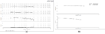
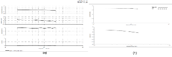
The magnitude, phase, coherence and error plots of the quad- rotor altitude model response obtained from the CIFER identi- fication is depicted in Fig. 5.6. The model shows excellent co- herence (ϒ2 ≈ 0.7) from 1 rad/sec up to 9 rad/sec, with both magnitude and phase constant to within 10% over excitation frequency range; hence this indicates a good model. The ex- perimental flight data is represented with a second order criti- cally damp system (Equation 25). Similarly, the magnitude of the identified model fits the experimental flight data from 0.1 rad/s to 1 rad/s, while the phase fits from zero rad/s to 1.2 rad /s as depicted in Fig. 4.
IJSER © 2014 http://www.ijser.org
International Journal of Scientific & Engineering Research, Volume 5, Issue 2, February-2014 803
ISSN 2229-5518
φ
![]()
∂u2
![]()
= 12.4s _ 8.7
s 2 + 15.8s + 10.2
e −0.245 s
(25)
Fig. 4. (a) Altitude model (b) model versus flight data fit.
The magnitude, phase, coherence and error plots of the quadrotor roll attitude response obtained from the CIFER identification depicted in Fig. 5a, shows excellent coherence (ϒ2 ≈ 0.7) from 1 rad/sec up to 12 rad/sec, with both magnitude and phase constant to within 1 % over excitation frequency range, hence indicates a good model. However, at 0.6 rad/s, there was a 90 degrees phase a rollover. The vehicle's roll response experimental flight data is
represented with a second order critically damp system (Equation
26). Similarly, the magnitude and phase of the identified model fits the experimental flight data from over the entire frequency
Fig. 6. Pitch attitude model (b) model versus flight data fit.
The magnitude, phase, coherence and error plots of the quad- rotor yaw attitude model depicted in Fig. 7a shows poor co- herence (ϒ2 <0.6 ) at lower and upper frequency, a good coher- ence over the middle frequency (ϒ2 >0.7) from 0.3 rad/sec up to 11.5 rad/sec having both magnitude and phase constant at within 5% over the frequency range. Hence, this indicates a good model. The vehicle's yaw response experimental flight data is represented with a second order critically damp system (Equation 28). Similarly, the magnitude and phase of the iden- tified model fits the experimental flight data from over the entire frequency range as depicted in Fig. 7b.
range as depicted in Fig. 5b.
ω
![]()
∂u1
![]()
= 28.7
s 2 + 863.5s + 250
e − 2.2 s
(28)
θ
![]()
∂u3
![]()
= 12.7s _ 6.7
s 2 + 16.2s + 8.2
e −0.267 s
(26)
Even though the single axis transfer-functions can accurately model the on-axis angular and vertical responses, the MIMO state-space models are needed to fully characterize the coupled dynamics of the quadrotor. The 6-DOF hover state-space model generated in the system identification process exhibited coupled dynamics between its responses to the inputs siganals. However, based on [15], the F and G matrices containing the stability and control derivatives were tuned by CIFER such that the model match those derived from the flight test data. The MIMO model shows a good agreement between the on-axis state-space model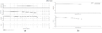
Fig. 5. Roll attitude model (b) model versus flight data fit.
Similar to the vehicle's roll attitude model, the magnitude, phase, coherence and error plots of the quadrotor pitch atti- tude model depicted in Fig. 6a, shows excellent coherence (ϒ2
≈ 0.7) from 1 rad/sec up to 12 rad/sec, with both magnitude and phase constant to within 1% over excitation frequency range. Hence, this indicates a good model; however, at 0.6 rad/s, there was a 90 degrees phase a rollover. The vehicle's roll response experimental flight data is represented with a second order critically damp system (Equation 27). The magni- tude and phase of the identified model fits the experimental flight data from over the entire frequency range as depicted in Fig. 6b.
and the transfer-functions control and damping derivatives. The
on-axis delays on the input control channels are as follows; a time delay of 0.254 rad/sec (Equation 25) on the roll channel,
0.267 rad/sec (Equation 26) on the pitch channel, 0.074 rad/sec (Equation 27) on the yaw channel, and 2.4 rad/sec (Equation 28) on the altitude channel. In the transfer function models, the gains are the control derivatives and the poles are the damping deriva- tive. The slight change in values occurs since the state-space model accounts for the simultaneous fit to the complete MIMO frequency responses. By and large, the models show excellent fit with the actual and predicted frequency reposnse which can be use for flight control system design.
This paper has presented the frequency-domain system identi-
ψ
![]()
∂u4
![]()
= 9.6s _ 28.8
s 2 + 16.1 + 7.3
e −0.0741s
(27)
fication of a quadrotor. The hover flight condition of the vehicle was considered as the reference flight operating point in extract- ing the vehicle's parameterized model using the CIFER software
IJSER © 2014 http://www.ijser.org
International Journal of Scientific & Engineering Research, Volume 5, Issue 2, February-2014 804
ISSN 2229-5518
package. The identification procedure started with the collection of the experimental time domain flight data. For each flight data record, the quadrotor was set to hover and a piloted frequency sweep excitation signal was applied to the four control variables, one after the other, with the bandwidth of the excitation signal ranged between 0.2 rad/sec – 20 rad/sec. While the frequency sweep was executed by the primary input of interest, the second- ary inputs were kept uncorrelated to maintain the vehicle near the reference operating point. A systematic selection procedure of the model structure for the parameterized transfer-function model and the state-space model was employed, with emphasis on the selection of stability and control derivatives included in the pa- rameterized state-space model. The extraction of the vehicle’s transfer-function model involved the determination of the struc- ture and order of the parameterized model, and the determination of the values of the model parameters using an optimization algo- rithm. The optimization algorithm was based on an iterative ro- bust secant algorithm that reduced the phase and magnitude error between the state space model and the flight data frequency re- sponses, the iteration was executed until the average of the se- lected frequency responses cost functions were minimized. Simi- larly, the parametric state-space model extraction involved an iterative procedure until the most suitable stability and control derivatives of the state-space model were selected based on the three accuracy metrics namely: frequency responses cost func- tions; percentage of the Cramér–Rao (CR) bound for each pa- rameter; percentage of the insensitivity of each parameter with respect to the cost function. The model of the quadrotor extracted possesses an excellent average cost functions value of 21 and produced physically reasonable values for the stability deriva- tives. Similarly, the MIMO model shows a reasonable agreement between the on-axis state-space model and the transfer-functions control and damping derivatives.
[1] M. Ryll, H. H. Bulthoff, and P. R. Giordano, “Modeling and control of a quadrotor uav with tilting propellers,” in proceedings of the IEEE International Conference on Robotics and Automation (ICRA), (Saint Paul, Minnesota, USA), pp. 4606-4613, May 2012.
[2] S. Bellens, J. D. Schutter, and H. Bruyninckx, “A hybrid pose / wrench control framework for quadrotor helicopters,” in proceed- ings of the IEEE International Conference on Robotics and Auto- mation (ICRA), (Saint Paul, Minnesota, USA), pp. 2266-2274, May
2012.
[3] L. Jun and L. Yuntang, “Dynamic analysis and pid control for a quadrotor,” in proceedings of the IEEE International Conference on Mechatronics and Automation, (China), pp. 573-578, August 2011.
[4] D. M. Ly and H. Cheolkeun, “Modeling and control of quadrotor mav using vision-based measurement,” in proceedings of the Inter- national Forum of Strategic Technology (IFOST), (Ulsan, South Korea), pp. 77- 75, October 2010.
[5] F. Wang, B. Xian, G. Huang, and B. Zhao. Autonomous hovering
control for a quadrotor unmanned aerial vehicle. In proceedings of the Control Conference (CCC), 2013, pages 620–625, 2013.
[6] F. Wang, B. Xian, G. Huang, and B. Zhao. Autonomous hovering control for a quadrotor unmanned aerial vehicle. In proceedings of the Control Conference (CCC), 2013, pages 620–625, 2013.
[7] I. E. Putro, A. Budiyono, K. J. Yoon, and D. H. Kim. Modeling of unmanned small scale rotorcraft based on neural network identifica-
tion. In proceeding of the IEEE International Conference on Robot- ics and Biomimetics, ROBIO, 2008, pages 1938–1943, 2009.
[8] D.H. Shim, Hyoun Jin Kim, and S. Sastry. Control system design for rotorcraft-based unmanned aerial vehicles using time-domain system identification. In proceedings of the IEEE International
Conference on Control Applications, 2000, pages 808–813, 2000.
[9] G. Zhengbang, F.Wei, G. Tongyue, and L. Jun. Modeling and iden- tification of a hovering sub-miniature rotorcraft. In International Symposium on Intelligent In- 41 Bibliography formation Technolo- gy Application Workshops, IITAW, 2008, pages 1104–1108, 2008.
[10] Y. S. Chang, B.I. Kim, and J. E. Keh. Rotorcraft dynamics model identification and hovering motion control simulation. In proceed- ings of the 34th IEEE Annual Conference on Industrial Electronics
(IECON), 2008, pages 366–370, 2008.
[11] M. B. Tischler. System identification requirements for high- bandwidth rotorcraft flight control system design. In American Control Conference, 1991, pages 2494–2502, 1991.
[12] I. A. Raptis and K. P. Valvanis. Linear and Nonlinear Control of
Small-Scale Unmanned Helicopters. Springer, 2011.
[13] L. L. Jung. System Identification: Theory for the User. Prentice
Hall, New York„ 1999.
[14] T. Soderstrom and P. Stoica. System Identification. Prentice Hall, New York„ 1989.
[15] M. B. Tischler and R. K. Remple. Aircraft and Rotorcraft System
Identification. AIAA Education Series (AIAA, Washington), 2006. [16] R. W. Ramirez. The FFT: Fundamentals and Concepts. Prentice
Hall, Upper Saddle River, NJ, 1985.
[17] J. S. Bendat and A. G. Piersol. Engineering Apllications of Correla- tion and Spectral Analysis, 2nd Edition. Wiley, New York, 1993.
[18] V. Klein and E. A. Moreli. Aircraft System Identification Theory and Practice, AIAA Education Series. AIAA, Washington, 2006.
[19] B. T. Mark and K. R. Robert. Aircraft and Rotorcraft System Iden- tication. AIAA, Virginia, USA, 2006.
[20] B. Mettler, M. B. Tischler, and T. Kanade. System identification of small-size unmanned helicopter dynamics. In proceedings of the
55th Forum of American Helicopter Society, May 1999.
[21] B. Mettler. Identification Modeling and Characteristics of Miniature
Rotorcraft. Kluwer Academic Publishers, Norwel, 2003.
[22] B. Mettler, T. Kanade, and M. B. Tischler. System identification modeling of a model-scale helicopter, technical report. Technical report, Carnegie Mellon University, 2000.
[23] C. Guowei, B. M. Chen, K. Peng, M. Dong, and T. H. Lee. Model- ing and control system design for a uav helicopter. In proceedings of the 14th Mediterranean Conference on Control and Automation,
2006, MED, 2006, pages 1–6, 2006.
[24] J. Gadewadikar, F. Lewis, K. Subbarao, and B. Chen. Structured h
infinity command and control loop design for unmanned helicop- ters. Journal of Guidance, Control and Dynamics, 31:1093–1102,
2008.
[25] A.S. Imam and R. Bicker. Design and construction of a small-scale rotorcraft uav system. International Journal of Engineering Science and Innovative Technology (IJESIT), Vol. 2, in Pres, 2014.
IJSER © 2014 http://www.ijser.org