G3(t),g3(t) c.d.f. and p.d.f. of repair time of partially failed unit
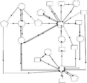
Fig:1. Transition Diagram
Profit Analysis of a Two Unit Standby Oil Delivering System with off line Repair Facility when Priority is given to Partially Failed Unit over the Completely Failed Unit for Repair and
System having a Provision of Switching over to
Another System
Rekha Narang, Upasana Sharma
Abstract— Profit analysis of two unit standby oil delivering system with three types of failure complete failure, normal to partial failure and partial to complete failure is analysed. Initially one unit is operative and the other is standby. In case of partial failure, repair of unit is done by switching off the unit. W hen both the units fail then for repairing, priority is given to partially failed unit over completely failed unit. The system is in down state if one unit is completely failed and other is partially failed On the complete failure of both the units there is a provision of switching over to the other similar system. This practical situation may be observed in an oil refinery plant. The system is analyzed by making use of semi-Markov processes and regenerative point technique.
Index Terms— Oil delivering system, Semi Markov process, Regenerative point technique, measures of system effectiveness and profit analysis.
In the field of reliability standby systems have been discussed by various researchers including [1-4] under various assump- tions/considerations. For graphical study, they have taken as- sumed valuesfor failure and repair rates, and not used the ob- served values. However, some researchers including [5-8] stu- died some reliability models collecting real data on failure and
repair rates of the units used in such systems. The concept of another line facility in case of failure of operating system has been introduced by Sharma et. al. [9]which can be seen in an oil refinery plant wherein on the failure of one standby oil delivering system, the supply is done by switching over to another system .This is done by changing a valve. A valve is a device which is used for switching over to another system. But the concept of three types of failures for such oil deliver- ing system has not been considered so far and in this paper authors have tried to bridge this gap. There may be situations where a unit may fail due to complete failure, normal to par- tial failure and partial to complete failure. On the complete failure of the operative unit, it is repaired or it’s component is replaced depending on the type of failure. In case of partial failure repair is done by switching off the unit and for repair of the units priority is given to partially failed unit over com-
pletely failed unit. The present study is based on the data col-
lected on the failure and repair rates for the oil delivering sys- tem working in the oil refinery plant.
Initially one unit is operative and the other is standby.
On the failure of the operative unit, it is repaired depending on type of failure or its component is replaced with a new one according as it is repairable or irreparable. The standby unit becomes operative at this stage If one unit is completely failed and other is partially failed unit then the system will be in down states and in the situation of complete failure of both the units, we switch over to the other system to avoid down time as the company may have other line facilities. Failure time is assumed to have exponential distribution. Re- pair/replacement times have been taken as arbitrary
s stand by
Fr unit is under repair
Fwr failed unit is waiting for repair
FR repair is continuing from previous state
Frep unit is under replacement
Fwrep failed unit is waiting for replacement
Frs repair of failed units is kept under suspension
CV valve change for being connected
IJSER © 2011 http://www.ijser.org
rate of direct complete failure of main pump
1 failure rate of normal to partial failure
2 failure rate of partial to complete failure
α 1 repair rate of unit
i =
P(Ti > t) dt
0
α 2 replacement rate of unit
β rate of change of valve
p prob. that unit is under repair
q prob. that unit is under replacement
The unconditional mean time taken by a system to transits’ to
any regenerative state ‘j’ when time is counted from epoch of
entrance into state ‘i’ is mathematically stated as
*
p prob. of switching over to another line
q prob. of failure of switching over to another line
G1(t),g1(t) c.d.f. and p.d.f. of the repair time of unit. G2(t),g2(t) c.d.f. and p.d.f. of the replacement time of
mij
t d Qij (t )
0
qij
(s)
unit.
G3(t),g3(t) c.d.f. and p.d.f. of repair time of partially failed unit
Fig:1. Transition Diagram
4
16
5 β 17
(Pfr,pfwr) (FR,Fwr) (Frs,Fwr,cv) (Fr,Fwr,c)
λ2q
8 λpq1 g1(t) λpp1 g1(t ) 6
λ1 g3 (t) λ (Fr s,pfr ) λ1 λqq1 (FR,Fwr p)
λq λp g3 (t)
A transition diagram showing the various states of the sys- tem is shown in Fig 1. The epochs of entry into states 0, 1,
2,3,5,7,10,12,17,18,19 and20 are regenerative points. The
14 (PfR,Fwrp) 3
15
(Pfr,o) (PfR,Fwr) g3 (t)
7
1 (Fr,o) λpq1 (Frs,Fwrp,cv)
β
transition probabilities are given below:
p01 = pe - ( + 1 ) t dt p02 = q e - ( + 1 ) t dt p03 = 1 e - ( + 1 ) t dt
p10 = g1(t) e - ( + 1 ) t dt
λ1 g3 (t) g1 (t) λp g2 (t)
19
0
(o,s) (Frps,Fwr, c)
g3 (t) β
10
g2 (t)
9
1 8
(FRp,Fwr)
λq 20
(Frps,Fwr,cv) g1 (t)
p11(4) = p q1(e - ( + 1 ) t ©1)g1 (t) dt
g (t) β (Frps,Fwrp,c) g (t)
2 1
pq1
p14 = 1
1
p30 = g3 1
12
(Frps,Fwrp,cv) λqp1
g2 (t) λpp1 λpq1
2
13
p3,14 =
q
![]()
1
p
1 g
11
(FR p,Fwrp) (Frps,Pfr)
p3,1(15) =
p3,1,(15,16)![]()
1
1 g
Let i(t) be the c.d.f. of the first passage time from regenerative
p12
1 g 3 1
1 g 3 2
state i to a failed state .To determine the mean time to system![]()
=
2 1
![]()
p
1
![]()
2
failure (MTSF) of the system, considering the failed state as absorbing states. By probabilistic arguments, we obtain the following recursive relation for i(t) :![]()
p3,2,(14,16) = p 3,1(15,16)
q
0(t) = Q01(t) (s) 1(t) + Q02(t) (s) 2(t) + Q03(t) (s) 3(t)
1(t) = Q10(t) (s) 0(t) + Q14(t) + Q15(t) + Q16 (t) + Q17 (t) +
p3, (16) =
![]()
1
g
g
Q18
(t) (s) 8(t)
2 1 2(t) = Q20(t) (s) 0(t) + Q2,9 (t) + Q2,10 (t) + Q2,11(t) + Q2,12(t) + Q2,13(t) (s) 13(t)
3(t) = Q30(t) (s) 0(t) + Q3,3(16) (t) 3(t) + Q3,1(15)(t) (s) 1(t)
+ Q3,1(15,16)(t) (s) 1(t) + Q 3,2(14) (t) (s) 2(t) +
The mean sojourn time (i) in the regenerative state ‘i’ is given by
Q3,2(14,16)(t) (s) 2(t)
8(t) = Q8,1(t) (s) 1(t)
13(t) = Q13,2(t) (s) 2(t)
IJSER © 2011 http://www.ijser.org
Now the mean time to system failure (MTSF) when the system starts from state ‘0’ is
– p15) { (2 +19 p2,10 +20 p2,12 ) ( - p3,2(14) -p3,2(14,16)) – (1- p2,2(11) – p2,13 – p13,2 – p2,12 ) 3 } + (- p1,2(6)- p17 ) {( 2 +19 p2,10 +20 p2,12 ) (- p3,1(15) – p3,1(15,16)) – (- p2,1(9) – p2,10 ) 3}] + (1-p3,3(16)) [0 {(1-p11(4) –
1
* *(s) N
p18 – p15) (1-p2,2(11) – p2,13 – p13,2 –p2,12 ) - (-p1,2(6)- p17) (- p2,1(9) –
MTSF
![]()
lim 0
p2,10)} + p01 {( 1 +17 p15 +18 p17 )(1-p2,2(11) – p2,13 – p13,2 –p2,12 ) – (-
Where
s0 s D
p1,2(6)- p17 ) (2 + 19 p2,10 +20 p2,12 )} – p02 {(1 +17 p15 + 18 p17) (- p2,1(9) –p2,10 ) – (1-p11(4) – p18 – p15)
(2 +19 p2,10 +20 }]
N = 0 {(1-p33(16)) (1-p18) (1- p2,13)} + 2 [ {1-p18 p81}{ p02 (1-
p33(16)) + (p3,2(14) + p3,2(14,16)) p03}] + K3 {p03 (1-p18) (1-p2,13)} +
8 p18 (1-p2,13){(1-p3,3(16)) (1-p02) – p03 p30 – p03
(p3,2(14) + p3,2(14,16))} + 13 p2,13 (1-p18) { (1-p3,3(16)) (1-p01) –
p03 p30 - p03(p3,1(15) + p3,1(15,16))}
D = (1-p3,3(16)){ - p01p10 +1 – p18) (1- p2,13) – p02 p20 (1- p18)} – p03 { p10 (p3,1(15) + p3,1(15,16)) + p30 (1 - p18) (1- p2,13) + p20 (p3,2(14) + p3,2(14,16)) (1- p18)}
Let Ai(t) be the probability that the system is in up state at instant t given that the system entered regenerative state i at t=0. The availability Ai(t) is see to satisfy the following recur- sive relations:
A0(t) = M0(t) + q01(t) A1(t) + q02(t)A2(t) +q03A3(t)
D1 = 0 [ p10 {( - p2,1(9) –p2,10) (-p3,2(14)-p3,2(14,16)) - (1-p2,2(11) –p2,13 – p13,2 –p2,12 ) (-p3,1(15) – p3,1(15,16))}- p20 { (1-p11(4) – p18 – p15 ) (-p3,2(14)- p3,2(14,16)) – (-p1,2(6)- p17 ) (-p3,1(15) – p3,1(15,16))} + p30 { (1-p11(4) – p18 – p15 ) p2,2(11) – p2,13 – p2,12 ) – (- p1,2(6)- p17 ) ( - p2,1(9) – p2,10)}+ K1 [ p03 {( - p2,1(9) – p2,10) (-p3,2(14) - p3,2(14,16)) – (1- p2,2(11) – p2,13 – p2,12 ) (- p3,1(15) – p3,1(15,16))} + {p01 (1- p2,2(11) – p2,13 – p2,12) – p02( - p2,1(9) – p2,10)} (1- p3,3(16))]+ K2 [ p03 { (- p1,2(6)- p17) (- p3,1(15) – p3,1(15,16)) – (1- p11(4) – p18 – p15 )(- p3,2(14) - p3,2(14,16))} + (1- p3,3(16)) { (1- p11(4) – p18 – p15) p02 – (- p1,2(6)- p17 ) p01}] + K3 [ p03 { (1- p11(4) – p18 – p15)p2,2(11) – p2,13 – p2,12 ) – (- p1,2(6)- p17 ) ( - p2,1(9) –p2,10)} + 5 p20 p15[ {(- p3,2(14)- p3,2(14,16)) p03 - p02(1- p33(16))} + p30{- (1- p2,2(11) – p2,13 – p2,12 ) p03} + (1- p2,2(11) –p2,13 – p2,12 ){(1- p33(16))}] +7 p17 [-(-p3,1(15) – p3,1(15,16))p03p20 + ( - p2,1(9) – p2,10)p03p30 –( - p2,1(9) –p2,10) (1-p3,3(16)) + p01p20 (1- p3,3(16))] +8 [(-p3,2(14)-p3,2(14,16))p03 p20 – p02 p20 (1- p3,3(16)) –
(1- p2,2(11) – p2,13 – p2,12 ) p03 p30 +(1- p2,2(11) – p2,13 – p2,12) (1-
A1(t) = M1(t) + q10(t) A0(t) + q11(4)(t) A1(t) + q12(6) (t) A2 +
p3,3(16)
)] + 10
p2,10
[-(-p3,2(14)
-p3,2(14,16)
) p03
p10
+{p02
p10
- (-p1,2(6)-
q15(t) A5(t) + q17(t) A7(t) + q18(t) A8(t)
p17)}{1- p3,3(16)} + (- p1,2(6)- p17) p03 p30] + 12 p2,12 [(-p3,1(15) – p3,1(15,16))
A2(t) = M2(t) + q20(t) A0(t) +q2,1(9)(t) A1(t) + q2,2(11)(t) A2(t) +
p p – (1- p
– p – p ) p p
+{-p p
+ ( -p
– p – p
03 10
11(4) 18
15 03 30
01 10
1 11(4)
18 15
q2,10(t) A10(t)+ q2,12(t) A12(t) + q2,13(t) A13(t)
)}{1- p3,3(16)}] +13 p2,13[{p03 (-p3,1(15) – p3,1(15,16)) –p01(1- p3,3(16))}p10 –
A3(t) = M3(t) + q30(t) A0(t) + q3,1(15)(t)A1(t) + q3,1(16,15)A1(t) +
(1 - p11(4)
– p18
– p15
) p03
p30
+ (1- p11(4)
– p18
– p15
) {1- p3,3(16)
}] + 17
q3,2(14)A2(t) + q3,2(16,14)A2(t) + q3,3(16)(t) A3(t)
p15
[ p03
{p20
( - p3,2(14)
- p3,2(14,16)
) – p30
(1- p2,2(11)
– p2,13
– p2,12
) } +{(1
A5(t) = q5,17(t) A17(t)
A7(t) = q7,18(t) A18(t) A8(t) = q8,1(t) A1(t) A10(t) = q10,19(t) A19(t) A12(t) =q12,20(t) A20(t) A13(t) =q13,2(t) A2(t)
A17(t) = M17(t) + q17,1(t) A1(t) A18(t) = M18(t) + q18,2(t) A2(t) A19(t) = M19(t) + q19,1(t) A1(t) A20(t) = M20(t) + q20,2(t) A2(t) where
M0(t) = e - ( + 1 ) t
-p2,2(11) – p2,13 – p2,12) - p02 p20}{1 - p3,3(16)}] +18 [{-p20 (- p3,1(15) – p3,1(15,16)) + p30( - p2,1(9) – p2,10)} p03 + {p01p20 – ( - p2,1(9) – p2,10)}{1- p3,3(16)}] + 19 p2,10 [ {p02 p10 – (- p1,2(6)- p17 ) } {1 - p3,3(16)} + {p30 (- p1,2(6)- p17 ) – (-p3,2(14)-p3,2(14,16)) p10 } p03] +20 p2,12 [ {p10 (-p3,1(15) – p3,1(15,16)) – p30 (1-p11(4) – p18 – p15 ) } p03 +{ (1- p11(4) – p18 – p15) – p01p10} {1- p3,3(16)}]
Busy period analysis for repair time only = N2/D1
Busy period analysis for replacement time only = N3/ D1
Expected no of Replacements = N / D
4 1
![]()
M1(t) = e - ( + 1 ) t (t)
Expected no of visits by repairman = N / D
5 1
M2(t) = e - ( + 1 ) t (t)
Expected time during which operation is = N6/ D1![]()
M3(t) = e - ( + 1 ) t (t) + 1 ( e - ( + 1 ) t © e - 2 t )![]() (t ) M17(t) = (t)
(t ) M17(t) = (t)
M18(t) = (t) M19(t) = (t) M20(t) = (t) M8(t) = (t) M13(t) = (t)
In steady-state, availability of the system is given by
N
performed by some other system
Expected down time = N7/ D1
N2= p03[ W1 + W8 p18 + W17 p15 + W18 p17 {( - p2,1(9) – p2,10 ) (- p3,2(14)
- p3,2(14,16)) – (1- p2,2(11) – p2,13 – p2,12 ) (- p3,1(15) – p3,1(15,16))} – (1-p11(4)
– p18 – p15 ) { W13 p2,13 (- p3,2(14)-p3,2(14,16)) – (1- p2,2(11) – p2,13 – p2,12
) W3 } + (- p1,2(6) - p17 ) { W13 p2,13 (- p3,1(15) – p3,1(15,16)) – ( - p2,1(9) – p2,10 ) W3}] + (1- p33(16))[p01 { p01 { W1 + W8 p18 + W17 p15 +W18 p17 p7,18 (1 -p2,2(11) – p2,13 – p2,12 ) – (- p1,2(6) - p17 ) W13 p2,13} – p02 {
A0 lim s A![]()
* (s) 1
s0 0
1
W1 + W8 p18 + W17 p15 + W18 p17 p7,18 ( - p2,1(9) – p2,10 ) – (1-p11(4) –
A=N1/D1
where
p18
– p15
)W13
p2,13}]
N1 = p03[ (1 +17 p15 +18 p17 ){ (-p2,1(9) –p2,10 ) (- p3,2(14) - p3,2(14,16) ) -
N3 = W2 + W20 p2,12 +W19 p2,10 [ -p03 { (1-p11(4)
– p18 – p15 p5,17) (-
(1- p2,2(11) – p2,13 – p13,2 –p2,12 ) (- p3,1(15) – p3,1(15,16))} – (1-p11(4) – p18
p3,2
(14)
- p3,2(14,16)
) – (-p1,2(6)
- p17 ) (-p3,1
(15)
– p3,1
(15,16)
) }+ {1- p3,3(16)
}{ -
IJSER © 2011 http://www.ijser.org
p01 (- p1,2(6) - p17 ) + p02 (1- p11(4) – p18 – p15 }] D1 is already specified
N4= W2 + W20 p2,12 p2,20 +W19 p2,10 p10,19 { p2,0 + p2,1(9) + p2,2(11) + p2,12
+ p2,10} [ - p03 { (1 - p11(4) – p18 – p15)(-p3,2(14)-p3,2(14,16)) – (-p1,2(6)- p17
p7,18p18,2)(-p3,1(15) – p3,1(15,16)) }+ {1-p3,3(16)}{ -p01 (-p1,2(6)- p17 p7,18p18,2)
+ p02 (1-p11(4) – p18p8,1 – p15 p5,17p17,1)}]
N5 = (1-p3,3(16))( (1-p11(4) – p18 – p15)(1-p2,2(11) –p2,13 –p2,12 )- (-p1,2(6)- p17)( - p2,1(9) –p2,10)
N6 = p03 [( W17 p1,5 + w18 p1,7 ) {( - p2,1(9) –p2,10) (-p3,2(14)-p3,2(14,16))
–(1-p2,2(11) –p2,13 – p2,12 )(-p3,1(15) – p3,1(15,16))} – (1-p11(4) – p1,8 – p15 )
{( W20p2,12 +w19 p2,10 )(-p3,2(14)-p3,2(14,16)) } + (-p1,2(6)- p17 ) { ( W20p2,12
+w19 p2,10 ) (-p3,1(15) – p3,1(15,16))}] + { 1-p3,3(16)}[ p01 {( W17 p15 + w18
p17 ) (1-p2,2(11) –p2,13 –p2,12 ) – (-p1,2(6)- p17 ) ( W20p2,12 +w19 p2,10
) } –p02 { ( W17 p15 + w18 p17 ) ( - p2,1(9) –p2,10)
– (1-p11(4) – p18 – p15 )( W20p2,12 +w19 p2,10 ) }]
N7 = p03[D8p18{ ( - p2,1(9) –p2,10) (-p3,2(14)-p3,2(14,16))(-p3,2(14)-p3,2(14,16)) - (1- p2,2(11) –p2,13 p13,2 –p2,12 )(-p3,1(15) – p3,1(15,16))}-D13p2,13{ (1- p11(4) – p18p – p15 )(-p3,2(14)-p3,2(14,16))- (-p1,2(6)- p17 )(-p3,1(15) – p3,1(15,16))}] + {1- p3,3(16)}[p01 {D8 p18 (1- p2,2(11) –p2,13 –p2,12 ) – (-p1,2(6)- p17 p7,18)D13 p2,13} – p02{ D8 p18 ( - p2,1(9) –p2,10)- (1-p11(4) – p18 – p15 p5,17)D13p2,13}]
In steady-state, the expected profit per unit time incurred to the system is given by
Profit (P) = C0A0 C1B0 C2BR0 C3R0 C4 V0 C5AP0 – C6 D0
where
C0 = revenue per unit up time
C1 = cost per unit time for which repairman is busy for repair
C2 = cost per unit time for which repairman is busy for replacement
C3 = cost per unit of replacement
C4 = cost per visit of repairman
C5 = cost per unit time for which operation is performed by other system
C6 = cost per unit time for which system is down
The following particular case is considered for graphical in- terpretation
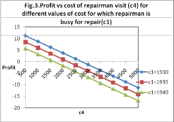
for different values of cost of repairman visit
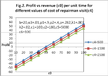
It can be interpretated from the graph that profit increases with increased in the value of revenue per unit up time(C0) and has lower values for higher values of cost of visit of re- pairman(C4)
1. For C4 = 500, the profit is positive or zero or negative according as C0 > or = or < 49.5616 and hence the rev- enue per unit up time should be fixed not less than
49.5616.
2. For C4 = 1500, the profit is positive or zero or negative according as C0 > or = or <54.1666 and hence the reve- nue per unit up time should be fixed not less than
54.1666
3. For C4 = 2500 the profit is positive or zero or negative according as C0 > or = or < 58.7717 and hence the rev- enue per unit up time should be fixed not less than
58.7717
Fig 3 shows the behavior of profit vs cost of repairman visit for different values of cost for which the repairman is busy for repair
g1(t) = 1 e 1 (t )
e 1 t
e 1 t
g1(t) = 2 e 2 (t ) e 1 t
g3(t) = 3 e 3 ( t )
;
e 1 t
c0=1000,c1=100 , c2=180 , c3=86390.19606 c4=500, c5=5000
Fig 2 shows the behavior of profit vs revenue per unit time
IJSER © 2011 http://www.ijser.org
It can be interpretated from the graph that profit decreses with increased in the value of cost of repairman visit(C4) and has lower values for higher values of cost for which the repairman is busy for repair(C1)
1. For C1 = 1930, the profit is positive or zero or negative according as C4 > or = or < 2752.4790 and hence the cost per visit of repairman should be fixed not be greater than 2752.4790
2. For C1 = 1935, the profit is positive or zero or negative according as C0 > or = or <2194.721 and hence the cost per visit of repairman should be fixed not be greater than 2194.721
3. For C1 = 1940 the profit is positive or zero or negative according as C0 > or = or < 1636.9852 and hence the cost per visit of repairman should be fixed not be greater than 1636.9852
So far as the profitability of the system is concerned, minimum amount of revenue and maximum amount to be paid to the repairman for repairing/replacing the failed unit can be suggested by the company using such sytem on the basis of the graphical interpretation given above.
The authors are thankful to Dr. G.Taneja for his valuable sug- gestions and the present paper is the outcome of his expe- rienced analytic outlook.
[1] R.K. Tuteja, and G.Taneja, “Profit analysis of one server one unit system with partial failure and subject to random inspection”, “Mi- croelectron. Reliab.”,vol 33,pp 319-322.1993.
[2] S.M. Gupta,N.K. Jaiswal,L.R. Goel,” Stochastic behavior of a two unit cold standby system with three modes and allowed down time”,”Microelectron Reliability”vol. 23,pp. 333-336.
[3] R.K.Tuteja, G.Taneja, and U.Vashistha, “ Two-dissimilar units system
wherein standby unit in working state may stop even without failure”, International Journal of Management and Systems”, vol 17 no
1,pp 77-100,2001
[4] Khaled, M.E.S. and Mohammed, S.E.S,. “Profit evaluation of two unit cold standby systemwith preventive and random changes in units.” Journal of Mathematics and Statistics. vol 1, pp. 71-77. 2005
[5] G.Taneja, V.K.Tyagi, and P. Bhardwaj,. “Profit analysis of a single unit programmable logic controller (PLC)”,” Pure and Applied Mathemati- ka Sciences”, vol. LX no (1-2),pp 55-71,2004
[6] G.Taneja, “Reliability and profit analysis of a system with PLC used as hot standby”. Proc.INCRESE Reliability Engineering Centre, IIT, Kharagpur India, pp: 455-464.,2005(Conference proceedings)
[7] B. Parasher, and G.Taneja,. “Reliability and profit evaluation of a standby system based on a master-slave concept and two types of repair facilities”. IEEE Trans. Reliabil., 56: pp.534-539, 2007
[8] Goyal, A. and D.V. Gulshan Taneja, 2009. Singh analysis of a 2-unit
cold standby system working in a sugar mill with operating and rest periods. Caledon. J. Eng., 5: 1-5.
[9] U.Sharma,Rekha, G Taneja., “ Analysis of a Two Unit Standby Oil Delivering System with a Provision of Switching Over to another System at Need to Increase the Availability”,”“ Journal of Mathematics and Statistics” vol 7 no 1 pp 57-60., 2011
IJSER © 2011 http://www.ijser.org