Preference will be given to the minor failure on the major one.
A repaired unit’s works as good as new.
International Journal of Scientific & Engineering Research, Volume 2, Issue 12, December-2011 1
ISSN 2229-5518
Profit Analysis of Two Unit Cold Standby System with Two Types of Failure under Inspection Policy and Discrete Distribution
Jasdev Bhatti, Ashok Chitkara, Nitin Bhardwaj
—————————— ——————————
Reliability is essential for proper utilization and maintenance of any system and equipments.Therefore it had gained much importance among manufacturers. Reliability deals with the development of new techniques for increasing the system effectiveness by reducing the frequency of failures and minimizing the high maintenance costs.A large literature exist in the area of reliability theory of standby systems.Many researchers had analyzed reliability models with failure and repair time by using continuous distribution.Aggarwal (2010) had considered the cold standby system with two types of failure using exponential distribution.Said, Salah, Sherbeny (2005) had analyzed the profit function for two unit cold standby system with preventive maintenance and random change in units.In this paper they considered the concept of inspection that is being performed after the failed unit get repaired by repairman to check the satisfactory result from repairman.Haggag (2009) had analyzed reliability models where the observed data were found to be large, for which the continous distribution was considered to be an accurate distribution.But it’s not always true as sometimes we come across some situations when the observed values are small. In such cases, continuous distribution might not adequately describe a discrete random variable. Then one has to deal reliability models with discrete distribution to obtain the various reliability measures of the system effectiveness such as the MTSF, availability and busy period of repairman etc.
In the field of reliability using discrete distribution Bhardwaj (2009) had analyzed two unit redundant systems with imperfect switching and connection time. In his research he had also analysed two identical unit standby and parallel systems with two types of failure.Gupta (2007) had studied two identical unit parallel systems with Geometric failure and repair time distributions. Now in this paper the two identical
coldstandby system was anzlyzed by introducing the concept
of inspection policy for detecting the two types of failure where inspection and repair time are taken as geometric
distribution. Initially one unit is operative and other is in cold standby. On the failure of a unit, an inspection is being done first to investigate the one out of two types (minor or major) of failures. This helps the repairman to repair an exact failure of the failed unit.Preference will be given to the minor failure on the major one. The repairman time taken by minor is less as compaired to major.
The model is analysed stochastically and the expressions for the various reliability measures of system effectiveness such as mean time to system failure, steady state availability, and busy period for both inspector and repairman were obtained.Graphs were also been drawn to analysed the behavior of MTSF and profit function with respect to repair and failure rate.
The following assumptions are associated with the model:
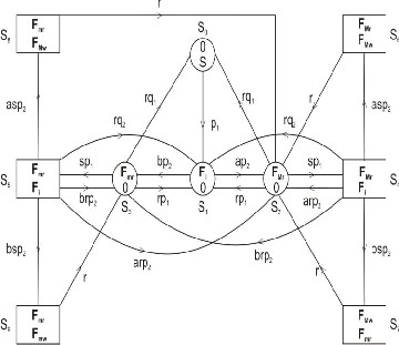
A system consists of two identical cold standby units arranged in a parallel network. Initially one unit is operative and other unit is in cold standby.
Upon the failure of an operative unit, the cold standby unit becomes operative instantaneously.
The system is assumed to be in the failed state when both units together were in failed conditions whether the cause of failure is major or minor.
A single repairman is available to repair both types of failed unit after being inspected.
IJSER © 2011 http://www.ijser.org
International Journal of Scientific & Engineering Research, Volume 2, Issue 12, December-2011 2
ISSN 2229-5518
Preference will be given to the minor failure on the major one.
A repaired unit’s works as good as new.
p [1 q (t 1) ]
ap [1 q (t 1) ]
Q01 (t) =
Q13 (t) =
1 1
1 q1
bp [1 q (t 1) ]
1 q
Q12 (t) =
2 2
1 q2
2
rq [1 (q s)t 1 ]
Q20 (t) = Q30 (t) =![]()
1 1
1 q1s
rp [1 (q s)t 1 ]
Q21(t) = Q31(t) = 1 1
1 q1s
sp [1 (q s)t 1 ]
Q24(t) = Q35(t) =
1 q1s
t 1
S0 = (O, S),
Q (t) = Q
(t) =![]()
rq2 [1 (q2 s) ]
S1 = (Fi, O),
S2 = (FMr, O),
41 51
1 q2 s arp [1 (q
s)t 1 ]
S3 = (Fmr, O)
Q42(t) = Q52(t) = 2 2
1 q2 s
brp [1 (q
s)t 1 ]
S4 = (FMr, Fi),
Q43(t) = Q53(t) = 2 2
1 q2 s
S5 = (Fmr, Fi),
asp [1 (q
s)t 1 ]
S6 = (FMr, FMw), S7 = (FMw, Fmr),
Q46(t) = Q58(t) =
2 2
1 q2 s
S8 = (Fmr, FMw),
bsp [1 (q
s)t 1 ]
S9 = (Fmr, Fmw).
Q47(t) = Q59(t) =
2 2
1 q2 s
IJSER © 2011 http://www.ijser.org
International Journal of Scientific & Engineering Research, Volume 2, Issue 12, December-2011 3
ISSN 2229-5518
Q62 (t) = Q72 (t) = Q82 (t) = Q93 (t) =
r[1 s( t 1) ]
![]()
1 s
Taking geometric transformation on both sides, we get
N (h)
(30-33)
(1-12)
The steady state transition probabilities from state Si to Sj can
R (h) 1
D1 (h)
The mean time to system failure is
be obtained from
Pij = lim Qij
i = lim![]()
N1 (h)
![]()
1 N1
It can be verified that
P01 = 1, P12+ P13 = 1,
t
where
h 1 D1 (h) D1
(34)
P20 + P21 + P24 = 1, P30 + P31 + P35 = 1,
P41 + P42 + P43 + P46 + P47 = 1, P51 + P52 + P53 + P58 + P59 = 1
P62 = P72 = P82 = P93 = 1
(13-19)
N1 = (0 -1) (1- P21) + 1 + 2 + P20 = 0 (1- P21) + 1 + 2 - P24
D1 = 1 P20 P21 = P24
(35-36)
Let Ai(t) be the probability that the system is up at epoch t when it is initially started from regenerative state Si by simple probabilistic argument the following recurrence relations are
Let Ti be the sojourn time in state Si (i = 0, 1, 2, 3, 4, 5, 6, 7, 8, 9),
then mean sojourn time in state Si is given by
obtained.
A0(t) = Z0(t) + q01(t1) A1(t1)
1 1 12
1) A2(t1) + q13(t1) A3(t1)
i E(Ti ) P(Ti t)
A (t) = Z (t) + q (t
so that
1
t 0
1 1
A2(t) = Z2(t) + q20(t1) A0(t1) + q21(t1) A1(t1)
+ q24(t1) A4(t1)
A3(t) = Z3(t) + q30(t1) A0(t1) + q31(t1) A1(t1)![]()
0 = ,
1 q1
1
![]()
1 = ,
1 q2
![]()
2 = 3 = ,
1 q1s
1
+ q35(t1)A5(t1)
A4(t) = q41(t1) A1(t1) + q42(t1) A2(t1)+ q43(t1) A3(t1)
+ q46(t1) A6(t1)+ q47(t1) A7(t1)![]()
4 = 5 = ,
1 q2 s
6 = 7 = 8 = 9 =![]()
1 s
(20-24)
A5(t) = q51(t1) A1(t1) + q52(t1) A2(t1)+ q53(t1) A3(t1)
+ q58(t1) A8(t1)+ q59(t1) A9(t1) A6(t) = q62(t1) A2(t1)
A7(t) = q72(t1) A2(t1)
Mean sojourn time (mij) of the system in state Si when the
system is to transit into Sj is given by
A8(t) = q82(t1) A2(t1) A9(t) = q93(t1) A3(t1)
(37-46)
mij = t qij (t)
By taking geometric transformation and solving the equation
t 0
N (h)
m01 = q10, m12 + m13 = q21,
m20 + m21 + m24 = m30 + m31 + m35 = sq1 2,
and
A (h) 2
D2 (h)
m41 + m42 + m43 + m46 + m47 = m51 + m52 + m53 + m58 + m59 = sq2 4
m62 = m72 = m82= m93 = s 6
(25-29)
Z0(t) = q1t , Z1(t) = q2t , Z2(t) = Z3(t) = (q1s)t, Z4(t) = Z5(t) = (q2s)t Z6 (t) = Z7 (t) = Z8 (t) = Z9 (t) = st
Hence,
(47)
Let Ri(t) be the probability that system works satisfactorily for
atleast t epochs ‘cycles’ when it is initially started from
Z i (h) = i
The steady state availability of the system is given by
operative regenerative state Si (i = 0, 1, 2, 3). R0(t) = Z0(t) + q01(t 1) R1(t1)
A0 =
lim A0 (t)
t
R1(t) = Z1(t) + q12(t1) R2(t1) + q13(t1) R3(t1)
R2(t) = Z2(t) + q20(t1) R0(t1) + q21(t1) R1(t1) R3(t) = Z3(t) + q30(t1) R0(t1) + q31(t1) R1(t1)
Hence, by applying ‘L’ Hospital Rule, we get
IJSER © 2011 http://www.ijser.org
International Journal of Scientific & Engineering Research, Volume 2, Issue 12, December-2011 4
ISSN 2229-5518
A0 = -![]()
N 2 (1)
B0 =
lim B0 (t)
t
D2 (1)
(48)
Hence, by applying ‘L’ Hospital Rule, we get
N3 (1)
![]()
B0 = -
where
N2 (1) = 0P20 (1 – P24P47) + 1 {1 – P24 + P24P41}(1 – P24P47)
+2(1 – P24P47)
where
D2 (1)
(61)
D2 (1) = {q10 P20 (1 – P24P47) + q21 [1–P24 + P24P41] (1 – P24P47)
+ sq12(1 – P24P47) + sq24 P24 (1 – P24P47)
+ s6P24 [P46 + P47] (1 – P24P47)}
(49-50)
N3(1) = 1 {1 – P24 + P24P41}(1 – P24P47)+4 P24(1 – P24P47).
and D2 (1) is the same as in availability analysis.
(62)
Now, the expected uptime of the system at epoch t is given by
Let
B' (t) be the probability that the repair facility is busy in
up(t) =
t
x 0
A0 (x)
repairing of failed unit when the system initially starts from regenerative state Si. Using simple probabilistic arguments, the following recurrence relations can be easily developed.
so that
(h) A0 (h)
B' (t)
' ( )
= q01(t1) B1 (t 1)
' '
![]()
up 1 h
B1 t
= q12(t1) B2 (t 1) + q13(t1) B3 (t 1)
B' (t) = Z2(t) + q20(t1) B' (t 1) + q21(t1) B' (t 1)
2 0 1
+ q24(t1) B' (t 1)
4
B' (t) = Z3(t) + q30(t1) B' (t 1) + q31(t1) B' (t 1)
Let Bi (t) be the probability of the inspector who inspect the 3 0 1
'
kind of failure of a failed unit before being repaired by
repairman. Using simple probabilistic arguments, as in case of
' ( )
+ q35(t1) B5 (t 1)
' '
B4 t
= Z4(t) + q41(t1) B1 (t 1) + q42(t1) B2 (t 1)
reliability and availability analysis the following recurrence ' '
relations can be easily developed. B0(t) = q01(t1) B1(t1)
+ q43(t1) B3 (t 1) + q46 (t1) B6 (t 1)
+ q47 (t1) B7 (t 1)
B1(t) = Z1(t) + q12(t1) B2(t1) + q13(t1) B3(t1)
' ( )
51
B' t
+ q52(t1) B (t 1)
B2(t) = q20(t1) B0(t1) + q21(t1) B1(t1)+ q24(t1) B4(t1)
B5 t
= Z (t) + q
(t 1)
1 ( 1) 2
B3(t) = q30(t1) B0(t1) + q31(t1) B1(t1)+ q35(t1) B5(t1)
+ q53(t1) B' (t 1) + q58 (t1) B' (t 1)
B4(t) = Z4(t) + q41(t1) B1(t1) + q42(t1) B2(t1)
+ q43(t1) B3(t1+ q46 (t1) B6 (t1)
+ q59
'
3 8
(t1) B' (t 1)
'
+ q47 (t1) B7 (t1)
B6 (t) = Z6(t) + q62(t1) B2 (t 1)
B5(t) = Z5(t) + q51(t1) B1(t1) + q52(t1) B2(t1)
B' (t) = Z7(t) + q
72(t1)
B' (t 1)
+ q53(t1) B3(t1) + q58 (t1) B8 (t1) 7 2
' '
+ q59 (t1) B9 (t1)
B8 (t) = Z8(t) + q82(t1) B2 (t 1)
B6(t) = q62(t1) B2(t1)
B' (t) = Z (t) + q
(t1) ' ( 1)
B7(t) = q72(t1) B2(t1) B8(t) = q82(t1) B2(t1)
9 9 93
B3 t
(63-72)
B9(t) = q93(t1) B3(t1)
(51-60)
By taking geometric transformation and solving the equation![]()
B ' (h) N 4 (h)
By taking geometric transformation and solving the equation
D2 (h)
![]()
B (h) N 3 (h)
D2 (h)
The probability that the repair facility is busy in repairing the failure of failed unit is given by
The probability that the inspection facility is busy in inspecting the failure of failed unit is given by
B ' =
lim
t
B' (t)
Hence, by applying ‘L’ Hospital Rule, we get
IJSER © 2011 http://www.ijser.org
International Journal of Scientific & Engineering Research, Volume 2, Issue 12, December-2011 5
ISSN 2229-5518
where
B ' = -
![]()
N 4 (1)
D2 (1)
(73)
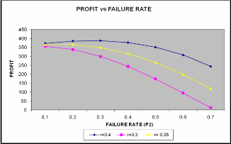
For r = 0.4, profit function P > or = or < 0 as the failure rate p2 < or = or > 0.954. So the system is preferable only if the failure rate is less than 0.954
(r) for different values offailure rate (p2). It appears from
N4(1) = 2 (1 – P24P47)+ 4 P24(1 – P24P47)
+ 6P24 [ P46 + P47](1 – P24P47)
and D2 (1) is the same as in availability analysis.
The expected total profit in steady-state is
P = C0A0 C1 B0 – C2 B '
where
C0: be the per unit up time revenue by the system
(74)
(75)
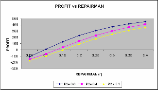
graph that Profit increases with increase in repair rate. Following observations have also been observed from the graph:
For p2 = 0.3, profit function P > or = or < 0 as the repair
rate r > or = or < 0.151. So the system is preferable only if the repair rate is greater than 0.151.
For p2 = 0.4, profit function P > or = or < 0 as the repair rate r > or = or < 0.125. So the system is preferable only if the repair rate is greater than 0.125.
For p2= 0.6, profit function P > or = or < 0 as the repair rate r > or = or < 0.0578. So the system is preferable
system
C1 & C2: be the per unit down time expenditure on the
only if the repair rate is greater than 0.0578.
The behaviour of the MTSF and the profit function w.r.t failure rate and repair rate have been studied through graphs by fixing the values of certain parameters a, b, C0 , C1 and C 2 as
a = 0.4, b = 0.6, C0 = 400, C1 = 100 and C2 = 200. On the basis of the numerical values taken as: P = 122.9535, r = 0.15 and s = 0.85
The values of various measures of system effectiveness are obtained as:
Figure: 2 show the behavior of MTSF w.r.t failure rate (p2).It appears from graph that MTSF decreases with increase in failure rate.
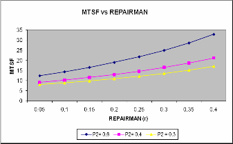
appears from graph that MTSF increases with increase in repair rate.
(p2) for different values of repair rate (r). It appears from graph that Profit decreases with increase in failure rate. Following observations have also been observed from the graph:
For r = 0.3, profit function P > or = or < 0 as the failure
rate p2 < or = or >0.721. So the system is preferable only if the failure rate is less than 0.721.
For r = 0.35, profit function P > or = or < 0 as the failure rate p2 < or = or >0.811. So the system is preferable only if the failure rate is less than 0.811.
This paper concluded that the preventive maintenance of units increases both the availability and profit of the system by providing the numerical results for MTSF, availability and busy period of repairman and inspector. It also provides information for other researchers and companies following such systems to prefer the equipments which satisfied the conditions as discussed.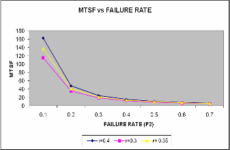
IJSER © 2011 http://www.ijser.org
International Journal of Scientific & Engineering Research, Volume 2, Issue 12, December-2011 6
ISSN 2229-5518
Jasdev Bhatti
Research Scholar,
Chitkara University, Himachal Pradesh, India.
Ashok Chitkara
Chancellor,
Chitkara University, Himachal Pradesh, India.
Nitin Bhardwaj
Asst. Professor,
Royal Institute of Management & Technology,
characteristic of cold-standby redundant syatem‛,
May 2010 3(2), IJRRAS.
Involving Common Cause Failures and Preventive
Maintenance‛, J.Math & Stat., 5(4):305-310, 2009, ISSN
1549-3644.
system with imperfect switching and connection time‛, International transactions in mathematical sciences and Computer,July-Dec. 2009,Vol. 2, No. 2, pp. 195-202.
analysis of a single unit redundant system with two kinds of failure and repairs‛, Reflections des. ERA- JMS, Vol. 3 Issue 2 (2008), 115-134
parallel syatem with Geometric failure and repair time distributions‛, J. of comb. Info. & System Sciences, Vol. 32, No.1-4, pp 127-136 (2007)
analysis fof a two unit cold standby system with preventive maintenance and random change in Units‛, 1(1):71-77, 2005, ISSN 1549-3644 (2005).
IJSER © 2011 http://www.ijser.org
International Journal of Scientific & Engineering Research, Volume2, Issue 12, December-2011 7
ISSN 2229-5518
Sonepat, Haryana,lndia.
IJSER ©2011 http //www 11ser org