International Journal of Scientific & Engineering Research, Volume 6, Issue 4, April-2015 1876
ISSN 2229-5518
Phonon Dispersion and Heat Capacity in Poly N- Isopropylacrylamide
Rushi Ghizal, Ghazala .R .Fatima, Seema Srivastava
Abstract—A study of the normal modes of vibration and their dispersion in Poly N-Isopropylacrylamide (PNIPAm) based on the Urey–Bradley force field is reported. It provides a detailed interpretation of IR and Raman spectra. Characteristic feature of dispersion curves such as regions of high density-of- states, repulsion and character mixing of dispersive modes are discussed. Predictive values of heat capacity as a function of temperature are calculated.
Keywords—Dispersion curves, Density-Of-States, Heat Capacity, Normal Modes, Phonon Dispersion, Poly N-Isopropylacrylamide, Vibrational
Dynamics.
1 INTRODUCTION
—————————— ——————————
Poly N-Isopropylacrylamide is a temperature-sensitive polymer. It exhibits a sharp phase transition close to 320 C. When heated in water above this temperature it undergoes a reversible phase transition from a swollen hydrated, coil conformation to a sunken dehydrated, globule transition [1]. Since PNIPAm expels it’s liquid content at a temperature near that of the human body, it has a great potential for application in tissue engineering [2],[3], drug delivery [4],[5],[6] , switches [7].
Sami Makharza, et al [8] have reported the FT-IR spectra
of PNIPAm in water. A large number of studies like FTIR
spectra [9],[10], Raman spectra [11], electronic spectra [12], synthesis [13],[14], have been made. None of the spectroscopic studies contain dispersion curves. In general the IR absorption, Raman spectra & Inelastic Neutron Scattering from polymeric systems are very complex and cannot be unraveled without the full knowledge of dispersion curves. Dispersion curves also give information on the extent of coupling along the chain and dependence of the frequency of a given mode upon the sequence length of ordered conformation. Thus the study of phonon dispersion in polymeric systems constitutes to be of topical importance.
In the present work we report a complete normal mode analysis of PNIPAm (Fig.1a) using Urey-Bradley force field which in addition to valence force field accounts for the intra-unit nonbonded and tension terms. The FT-IR spectra reported by Sami Makharza, et al [8] have been used. The density of states obtained from the dispersion curves is
used to calculate the heat capacity of PNIPAm in the
Fig 1a Chemical repeat unit of PNIPAm.
2 METHOD
2.1 Normal mode calculation
The calculation of normal mode frequencies has been carried out according to well known Wilson’s GF matrix [15] method as modified by Higg’s [16]. It consists of writing the inverse kinetic energy matrix G and the potential energy matrix F in terms of internal co-ordinates which are infinite in number. However due to screw symmetry of the polymer, a transformation similar to that given by Born and Von Karman can be performed. It reduces the infinite problem to finite dimensions [17]. The vibrational secular equation, which gives normal mode frequencies and their dispersion as a function of phase angle, has the form:
[G(δ)F(δ) − λ(δ)I] = 0, 0 ≤ δ ≤ π (1)
The vibrational frequencies ν(δ)(in cm-1) are related to the
eigen values λ(δ) by the following relation:
λ(δ) = 4π2 c2ν2(δ) (2)
A plot of νi (δ) verses 𝛿𝑖 R gives the dispersion curve of i
temperature range 50-500 K.
th
mode. The frequencies obtained from this expression are in wave numbers.
2.2 Calculation of Specific heat
Dispersion curves can be used to calculate the specific heat of polymeric system. For a one-dimensional system the density-of-state function or the frequency distribution function expresses the way energy is distributed among the
IJSER © 2015 http://www.ijser.org
International Journal of Scientific & Engineering Research, Volume 6, Issue 4, April-2015 1877
ISSN 2229-5518
various branches of normal modes of the crystal and it can be calculated from the relation:
𝑔(𝜈) = ∑𝑗 �
(3)

𝜕𝜈𝑗�−1 
𝜕𝛿
ν j (δ)=ν
Fig 1b Energy minimized structure of PNIPAm.
3.1 Vibrational modes
A chemical repeat unit of PNIPAm (Fig. 1a), has 19 atoms per residue and hence there would be 19x3–4 = 53
With ∫ g (ν)j dνj = 1
The sum is over all branches j. Considering a solid as an
assembly of harmonic oscillators, the frequency distribution
g(ν) is equivalent to a partition function. The constant volume heat capacity Cν can be calculated from the Debye’s relation:
ℎ𝜈𝑗 2 𝑒𝑥𝑝�ℎ𝜈𝑗⁄𝑘𝑇�
normal modes of vibrations. The vibrational frequencies have been calculated for the value of δ varying from 0 to π in the steps of 0.05π. The optically active modes are those for which δ = 0, π. The four zero frequencies at δ=0 correspond to acoustic modes, three representing translation along the three axes and the fourth one is rotation around the chain axis.
The assignments have been made on the basis of

Cν = ∑𝑗 𝑔(𝜈𝑗 ) 𝑘𝑁𝐴 �
�
𝑘𝑇
�𝑒𝑥𝑝�ℎ𝜈𝑗⁄𝑘𝑇�−1�

2 (4)
potential energy distribution, band position, band shape,
band intensity. The Urey- Bradley force field, takes into
account interactions in both bonded and non-bonded
The constant volume heat capacity Cv ,given by the
equation is converted into constant pressure heat capacity
Cp using the Nerst-Lindemann approximation [18],[19].
𝐶 2 𝑇
atoms, is used for the calculations of vibrational frequencies. A satisfactory match of the calculated frequencies with the observed peaks in the FTIR spectra [8] has been obtained by varying the force constants. The force

Cp –C v = 3RA0 �
(5)
Where A0 is a constant often of a universal value [3.9 x
0 �
𝑣 𝑚
constants giving “best fit” at 𝛿=0 to the experimental data,
are given in Table 1. All vibrational modes along with their
potential energy distribution are given in Table 2 at δ = 0.0 and Table 3 at δ = 1.0 respectively.
10-3 (kmol)/J)] and 𝑇𝑚
temperature.
is the equilibrium melting
The (N-H) stretching vibration has been calculated at
3295 cm-1 showing good agreement with the observed band also at 3296 cm-1. The frequencies calculated at 1649 cm-1 are
3 RESULT AND DISCUSSION
Molecular modeling technique (CS-Chemdraw) has been used to determine the structure of PNIPAm (Fig. 1b). It calculates the interatomic distances of atoms over all ranges of dihedral angles which are of interest. After this one selects a set of contact distance for the various kinds of atoms which are fully allowed and another which are considered minimal. The fully allowed contact distances result in fully allowed regions of conformational space. In other words, the minimal contact distances result in limiting the region of conformational space. Thus all unfavorable steric overlaps are excluded from consideration.
mainly due to (C=O) in combination with the contribution from (C-C) stretching and (C-N-H) angle bend. Again these are in agreement with the calculated value at 1648 cm-1 .The angle bend for (H-C-H) have been calculated at 1461 cm-1 and the observed value is also 1461 cm-1.
TABLE 1
INTERNAL COORDINATES AND FORCE CONSTANTS
IJSER © 2015 http://www.ijser.org
International Journal of Scientific & Engineering Research, Volume 6, Issue 4, April-2015 1878
ISSN 2229-5518
TABLE 2
VIBRATIONAL MODES OF PNIPAm AT δ = 0.0


Cal Obs. % of Potential Energy Distribution at δ = 0.0 Cal Obs. % of Potential Energy Distribution at δ = 0.0
3295 3296 ν(N-H)(100)
3057 3062 ν(C-H)(99)
3056 3062 ν(C-H)(99)
3030 ν(C-H)(99)
3028 ν(C-H)(99)
3027 ν(C-H)(98)
3027 ν(C-H)(100)
3014 ν(C-H)(96)
2966 2976 ν(C-H)(99)
2950 2968 ν(C-H)(99)
2892 2875 ν(C-H)(99)
1649 1648 ν(C-O)(70) + φ(C-N-H)(8) + ν(C-C)(5)
1549 1539 φ(C-N-H)(62) + ν(C-N)(18) + ν(C-N)(20)
1465 1461 φ(H-C-H)(93) + φ(H-C-C)(5)
1463 1461 φ(H-C-H)(95)
1461 1461 φ(H-C-H)(95)
1461 1461 φ(H-C-H)(95)
1453 1454 φ(H-C-H)(62) + φ(H-C-C)(19) + φ(H-C-C)(114)
1384 1391 φ(H-C-C)(47) + φ(H-C-H)(42) + ν(C-C)(10)
1382 1391 φ(H-C-C)(46) + φ(H-C-H)(42) + ν(C-C)(11)
1305 1305 φ(H-C-C)(57) + ν(C-C)(30)
1290 1281 φ(H-C-N)(32) + ν(C-N)(130) + φ(H-C-C)(9) +
φ(H-C-C)(8) + ν(C-C)(8)
1235 1242 ν(C-C)(37) + ν(C-N)(12) + φ(H-C-C)(12) +
φ(H-C-N)(12) + φ(C-N-H)(11)
1206 1219 ν(C-C)(30) + φ(H-C-C)(22) + ν(C-N)(110) +
φ(H-C-N)(9) + φ(C-N-H)(6) + φ(H-C-C)(15)
1168 1172 ν(C-C)(36) + φ(H-C-C)(34) + φ(H-C-C)(11) +
φ(C-C-N)(7)
1138 1133 ν(C-C)(29) + φ(H-C-C)(25) + φ(H-C-N)(9) +
ν(C-N)(8) + ν(C-N)(17) + φ(H-C-C)(5)
1046 φ(H-C-C)(34) + φ(H-C-C)(124) + ν(C-C)(15) +
φ(H-C-C)(7) + ν(C-N)(6)
1018 1023 φ(H-C-C)(72) + ν(C-C)(8) + φ(H-C-C)(7)
976 969 φ(H-C-C)(40) + φ(H-C-C)(34) + ν(C-C)(15)
960 969 φ(H-C-C)(21) + ν(C-C)(20) + φ(H-C-C)(119) +
φ(H-C-C)(11) + ν(C-N)(11)
917 929 φ(H-C-C)(75) + φ(H-C-C)(14)
911 906 φ(H-C-C)(43) + φ(H-C-C)(118) + ν(C-N)(115) +
φ(H-C-C)(6) + ν(C-N)(5)
900 906 φ(H-C-C)(63) + ν(C-C)(29)
891 890 φ(H-C-C)(135) + φ(H-C-C)(16) + ν(C-N)(11) +
ν(C-C)(7) + ν(C=O)(5)
819 820 φ(H-C-C)(35) + ω(C=O)(18) + ω(C-H)( 6) +
ν(C-C)(56)
772 782 ν(C-C)(69) + φ(H-C-C)(11)
720 726 ω(C=O)(21) + φ(O=C-N)(14) + φ(C-C-C)(9) +
φ(C-N-C)(9) + ν(C-C)(8) + φ(C-C-N)(6) +
φ(H-C-C)(5) + φ (H-C-C)(5) + ω(N-H)(5)
687 695 φ(H-C-C)(26) + ν(C-C)(23) + ω(C=O)(20) +
ω(N-H)(9) + ω(C-H)(5)
661 656 ν(C-C)(42) + φ(C-C-C)(24) + φ(H-C-C)(9) +
ω(C=O)(6) + ω(N-H)(6)
565 555 φ(H-C-C)(36) + φ(H-C-H)(15) + φ(C-C-C)(14) +
φ(H-C-C)(114)
509 516 ω(N-H)(43) + ω(C=O)(27) + φ(C-C-N)(17)
440 445 φ(C -C-N)(23) + φ(C-C-O)(16) + φ(O=C-N)(15) +
φ(H-C-C)(14) + ν(C-N)(6)+ φ(C-N-C)(5)
424 414 φ(C-C-C)(34) + φ(C-C-N)(19) + φ(H-C-C)(11) +
ν(C-C)(7) + φ(H-C-C)(15)
351 φ(C-C-N)(66) + ω(N-H)(28)
331 φ(C-C-C)(69) + φ(C-C-N) (14) + φ(H-C-C)(6)
247 φ(C-C-C)(38) + φ(C-C-O)(16) + ν(C-C)(9) +
φ(C-C-N)(8) + φ(O=C-N)(8) + φ(H-C-C)(8)
202 φ(H-C-C)(37) + φ(C-C-C)(27) + ω(C-H)(17) +
τ(C-C)(6)
141 φ(C-C-N)(28) + φ(C-C-C)(23) + ν(C-C)(14) +
φ(O=C-N)(9) + φ(H-C-C)(6)
128 φ(C-N-C)(34) + φ(C-C-N)(19) + φ(C-N-H)(11) +
φ(H-C-C)(11) + φ(C-C-C)(8) + ν(C-C)(7)
51 τ(C-C)(97)
50 τ(C-C)(99)
33 τ(C-N)(86) + τ(C-C)(10)
22 τ(C-C)(45) + τ(C-N)(31) + φ(C-C-C)(15)
10 τ(C-N)(64) + τ(C-C)(22) + φ(C-C-C)(8)
8 τ(C-C)(86) + τ(C-N)(13)
1 φ(C-C-N)(23) + φ(C-C-O)(21) + φ(H-C-C)(17) +
φ(O=C-N)(11) + ω(C-H)(9) + φ(H-C-N)(8)
0 φ(H-C-H)(51) + φ(H-C-C)(47)

IJSER © 2015 http://www.ijser.org
International Journal of Scientific & Engineering Research, Volume 6, Issue 4, April-2015 1879
ISSN 2229-5518
TABLE 3
VIBRATIONAL MODES OF PNIPAm AT δ = 1.0


Cal Obs. % of Potential Energy Distribution at δ = 1.0 Cal Obs. % of Potential Energy Distribution at δ = 1.0
3295 3296 ν(N-H)(100)
3057 3062 ν(C-H)(99)
3056 3062 ν(C-H)(99)
3030 ν(C-H)(99)
3028 ν(C-H)(99)
3027 ν(C-H)(98)
3027 ν(C-H)(100)
3014 ν(C-H)(96)
2957 2968 ν(C-H)(99)
2951 2968 ν(C-H)(99)
2892 2875 ν(C-H)(99)
1650 1648 ν(C=O)(70)+ φ(C-N-H)(6)+ ν(C-C)(5)
1549 1539 φ(C-N-H)(62)+ ν(C-N)(18)+ν(C-N)(10)
1465 1453 φ(H-C-H)(93) +φ(H-C-C)(5)
1463 1453 φ(H-C-H)(95)
1461 1453 φ(H-C-H)(78)+ φ(H-C-H)(10)
1461 1453 φ(H-C-H)(49)+ φ(H-C-C)(18) +φ(H-C-H)(16) +
φ(H-C-C)(11)
1461 1453 φ(H-C-H)(95)
1384 1375 φ(H-C-C)(47) +φ(H-C-H)(42) +ν(C-C)(10)
1382 1375 φ(H-C-C)(46) + φ(H-C-H)(42) +ν(C-C)(11)
1293 1281 φ(H-C-C)(34)+ν(C-C)(21)+ν(C-N)(11) +
φ(H-C-N)(11)
1288 1281 φ(H-C-C)(26) + φ(H-C-N)(23) + ν(C-N)(20) +
ν(C-C)(13) + φ(H-C-C)(6)
1224 φ(H-C-N)(22)+φ(C-N-H)(19)+ν(C-N)(17) +
φ(H-C-C)(12) +ν(C-N)(11) +ν(C-C)(8)
1168 1172 ν(C-C)(37)+φ(H-C-C)(33)+φ(H-C-C)(11) +
φ(C-C-N)(7)
1138 1133 ν(C-C)(34)+φ(H-C-C)(19)+φ(H-C-N)(9) +
ν(C-N)(8)+ν(C-N)(8)+φ(H-C-C)(6)
1118 1117 ν(C-C)(48)+φ(H-C-C)(20) +φ(H-C-C)(17)+
φ(C-C-C)(9)
1097 φ(H-C-C)(37)+ν(C-C)(26)+φ(H-C-C)(15) +
φ(H-C-H)(8)+φ(C-C-C)(5)
1018 1023 φ(H-C-C)(75) + ν(C-C)(7) + φ(H-C-C)(6)
988 φ(H-C-C)(25)+ν(C-N)(18)+φ(H-C-C)(15) +
ν(C-C)(13)+φ(C-C-C)(9)
976 969 φ(H-C-C)(39) +φ(H-C-C)(35)+ν(C-C)(15)
924 929 φ(H-C-C)(34)+φ(H-C-C)(31) +ν(C-N)(11)+
φ(H-C-C)(9)
917 906 φ(H-C-C)(77) +φ(H-C-C)(13)
901 906 φ(H-C-C)(57) +ν(C-C)(27) +φ(H-C-C)(6)
897 882 φ(H-C-C)(29)+φ(H-C-C)(28)+ν(C-C)(10)+
ν(C-N)(9) + ν(C-N)(8) + φ(H-C-C)(6)
824 820 φ(H-C-C)(28)+ω(C-H)(11)+ω(C=O)(10) + ν(C-C)(9) +φ(O=C-N))(8) +φ(C-N-C)(6) + φ(H-C-C)(5)
782 782 ν(C-C)(29)+φ(H-C-C)(16)+ φ(O=C-N)(11) +
ω(C=O)(8) +φ(C-N-C)(7)+ω(C-H)(5)
768 ν(C-C)(68)+φ(H-C-C)(11)+ν(C-N)(7)+
φ(H-C-C)(5)
708 711 ω(C=O)(44)+φ(H-C-C)(20)+ω(N-H)(15)+
ν(C-C)(9)
619 609 ν(C-C)(33)+φ(H-C-C)(18)+ω(N-H)(8) +
φ(C-C-C)(8) +φ(C-C-N)(5)
534 531 φ(H-C-C)(24)+ν(C-C)(20)+φ(C-C-N)(10)+ φ(H-C-H)(78)+φ(C-C-C)(7) +ω(N-H)(6) + φ(C-N-C)(5)
515 516 ω(N-H)(26)+ω(C=O)(15)+φ(H-C-C)(13)+
φ(C-C-C)(11)+ φ(C-C-N)(11) + φ(H-C-C)(10)
475 476 φ(C-C-C)(34)+ω(C=O)(13)+φ(C-C-N)(13)+
ω(N-H)(10) + φ(C-C-O)(8) +φ(H-C-C)(7)
414 414 φ(O=C-N)(23)+φ(H-C-C)(15)+φ(C-C-N)(15)+
φ(C-C-O)(9) +φ(C-C-C)(9)
351 φ(C-C-N)(65) +ω(N-H)(28)
336 φ(C-C-C)(62)+φ(C-C-N)(14)+φ(H-C-C)(7)+
ν(C-C)(6)
310 φ(C-C-C)(50)+φ(H-C-C)(10)+ν(C-C)(8)+
φ(C-C-O)(7) + φ(H-C-C)(7)+φ(H-C-H)(6)
248 φ(C-C-N)(32)+φ(C-C-C)(24)+ν(C-C)(15)+
φ(H-C-C)(7) + φ(C-C-O)(6)
164 φ(C-N-C)(31)+φ(C-C-N)(18)+ν(C-C-C)(15)+
φ(C-N-H)(10) + φ(H-C-C)(9)
54 τ(C-C)(32)+φ(C-C-C)(28)+φ(H-C-C)(12)+
τ(C-N)(8) + φ(C-C-N)(8)
51 τ(C-C)(97)
49 τ(C-C)(71) +φ(C-C-C)(10) +φ(H-C-C)(5)
34 τ(C-N)(54)+φ(C-C-C)(20)+τ(C-C)(7)+
φ(C-C-N)(5)
27 τ(C-N)(36)+φ(C-C-C)(24)+ω(C-H)(11)+
φ(H-C-C)(10) +τ(C-C)(9)
10 τ(C-N)(82) + τ(C-C)(5)
8 τ(C-C)(86) + τ(C-N)(13)
0.8 φ(C-C-N)(23)+φ(C-C-O)(21)+φ(H-C-C)(16)+
φ(O=C-N)(12)+ω(C-H)(10)+φ(H-C-N)(8)

3.2 Dispersion Curves
Dispersion curves provide information on the extent
and degree of coupling. They also help in the understanding of both symmetry-dependent and symmetry independent features. In general the IR absorption spectra and Raman scattering from polymeric systems are complex
and cannot be unraveled without the full knowledge of the dispersion curves. The regions of high density of state, which are observable in the IR and Raman spectra under suitable conditions, depend on the profile of the dispersion curves which play an important role in thermodynamical behavior of the system.
IJSER © 2015 http://www.ijser.org
International Journal of Scientific & Engineering Research, Volume 6, Issue 4, April-2015 1880
ISSN 2229-5518
The dispersion curves below 1600 cm-1 are shown in Fig.
2(a) and 3(a). The modes above 1600 cm-1 are either non
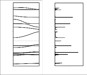
dispersive or their dispersion is less than 5 cm-1. A very interesting feature of the dispersion curve is convergence of various modes, i.e, the modes that are separated by a large wave number at the zone center come very close at the zone
boundary. This convergence arises mainly because of the
close sharing of potential energy in different measures by the various modes. For example, the two zone center wave modes calculated at 772 and 720 cm-1 are separated by 52 wave numbers at zone center, but at the zone boundary they are separated by only 14 wave numbers. Different
PED’S of both modes at different 𝛿 values are shown in
Table 4. Similar features are observed in pairs of modes,
which appear at zone center at 1138 and 1046 cm-1. These are separated by 92 wave numbers at zone center but are separated by 21 wave numbers at the zone boundary. Similar is the case for zone center modes at 1305 and 1289 cm-1.
1300
1200
1100
1000
900
800
0 0.5 1
Phase Factor (δ)
1300
1200
1100
1000
900
800
0 0.5 1
Density-of-states g(ν)
800
700
800
700
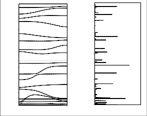
Fig 2b Dispersion curves of PNIPAm ( 800-1600 cm-1) and (b) density- of-states of PNIPAm (800-1600 cm-1).
600
600
500
500
400
400
300
300
200
200
100
100
0
0 Phas 0.5 tor (δ) 1
0
0 0.5 1
Density-of-states g(ν)
Fig 2a Dispersion curves of PNIPAm (0 – 800 cm-1) and (b) density-of- states of PNIPAm (0 – 800 cm-1).
TABLE 4
PAIR OF MODES SHOWING FEATURES OF DISPERSION CURVES

Before Exchange After Exchange


δ/π Freq PED δ/π Freq PED δ/π Freq PED δ/π Freq PED δ/π Freq PED

0.0 | 1206 | ν(C-C)(30)+ | 0.25 | 1197 | ν(C-C)(39)+ | 0.5 | 1174 | ν(C-C)(41)+ | 0.75 | 1168 | ν(C-C)(36)+ | 1.0 | 1168 | ν(C-C)(37)+ |
| | φ(H-C-C)(21)+ | | | φ(H-C-C)(25) | | | φ(H-C-C)(29) | | | φ(H-C-C)(32)+ | | | φ(H-C-C)(33)+ |
| | ν(C-N)1(10) | | | | | | | | | φ(H-C-C)M(11) | | | φ(H-C-C)M(11) |
0.0 | 1168 | ν(C-C)(36)+ | 0.25 | 1167 | ν(C-C)(36)+ | 0.5 | 1165 | ν(C-C)(38)+ | 0.75 | 1147 | ν(C-C)(37)+ | 1.0 | 1138 | ν(C-C)(34)+ |
| | φ(H-C-C)(34)+ | | | φ(H-C-C)(34)+ | | | φ(H-C-C)(33) | | | φ(H-C-C)(26) | | | φ(H-C-C)(19) |
| | φ(H-C-C)M(11) | | | φ(H-C-C)M(10) | | | | | | | | | |
0.0 | 976 | φ(H-C-C)M(40)+ | 0.25 | 976 | φ(H-C-C)M(40)+ | 0.5 | 976 | φ(H-C-C)M(40)+ | 0.75 | 981 | φ(H-C-C)M(19)+ | 1.0 | 987 | φ(H-C-C)M(14)+ |
| | φ(H-C-C)(34)+ | | | φ(H-C-C)(34)+ | | | φ(H-C-C)(33)+ | | | φ(H-C-C)(22)+ | | | φ(H-C-C)(24)+ |
| | ν(C-C)(15) | | | ν(C-C)(15) | | | ν(C-C)(15) | | | ν(C-C)(15)+ | | | ν(C-C)(12)+ |
| | | | | | | | | | | ν(C-N)(16) | | | ν(C-N)(18) |
0.0 | 960 | φ(H-C-C)M(21)+ | 0.25 | 961 | φ(H-C-C)M(22)+ | 0.5 | 967 | φ(H-C-C)M(21)+ | 0.75 | 975 | φ(H-C-C)M(36) | 1.0 | 976 | φ(H-C-C)M(39)+ |
| | φ(H-C-C)1(19)+ | | | φ(H-C-C)1(15)+ | | | φ(H-C-C)(16)+ | | | φ(H-C-C)(34)+ | | | φ(H-C-C)(35)+ |
| | φ(H-C-C)(11)+ | | | φ(H-C-C)(12)+ | | | ν(C-C)(19)+ | | | ν(C-C)(16) | | | ν(C-C)(14) |
| | ν(C-C)(20)+ | | | ν(C-C)(20)+ | | | ν(C-N)(14) | | | | | | |
| | ν(C-N)(11) | | | ν(C-N)(12) | | | | | | | | | |
IJSER © 2015 http://www.ijser.org
International Journal of Scientific & Engineering Research, Volume 6, Issue 4, April-2015 1881
ISSN 2229-5518
0.0 | 917 | φ(H-C-C)M(74)+ | 0.25 | 917 | φ(H-C-C)M(74)+ | 0.5 | 922 | φ(H-C-C)M(56)+ | 0.75 | 922 | φ(H-C-C)M(30)+ | 1.0 | 924 | φ(H-C-C)M(33)+ |
| | φ(H-C-C)(13) | | | φ(H-C-C)(13) | | | φ(H-C-C)(14)+ | | | φ(H-C-C)(11)+ | | | φ(H-C-C)1(30)+ |
| | | | | | | | φ(H-C-C)1(10) | | | φ(H-C-C)1(32) | | | ν(C-N)1(10) |
0.0 | 911 | φ(H-C-C)M(43)+ | 0.25 | 911 | φ(H-C-C)M(40)+ | 0.5 | 915 | φ(H-C-C)M(45) | 0.75 | 916 | φ(H-C-C)M(75)+ | 1.0 | 916 | φ(H-C-C)M(76)+ |
| | φ(H-C-C)1(18)+ | | | φ(H-C-C)1(20)+ | | | φ(H-C-C)1(22)+ | | | φ(H-C-C)(12) | | | φ(H-C-C)(12) |
| | ν(C-N)1(15) | | | φ(C-N)1(13) | | | φ(H-C-C)(12) | | | | | | |
0.0 | 900 | φ(H-C-C)M(63)+ | 0.25 | 900 | φ(H-C-C)(62)+ | 0.5 901 | φ(H-C-C)M(45)+ | 0.75 | 901 | φ(H-C-C)M(52)+ | 1.0 | 901 | φ(H-C-C)M(57)+ |
| | ν(C-C)(29) | | | ν(C-C)(29) | | ν(C-C)(20)+ | | | ν(C-C)(23) | | | ν(C-C)(26) |
| | | | | | | φ(H-C-C)1(15) | | | | | | |
0.0 | 891 | φ(H-C-C)1(35)+ | 0.25 | 894 | φ(H-C-C)1(34)+ | 0.5 898 | φ(H-C-C)M(39)+ | 0.75 | 897 | φ(H-C-C)M(34)+ | 1.0 | 896 | φ(H-C-C)M(28)+ |
| | φ(H-C-C)(16)+ | | | φ(H-C-C)(15)+ | | φ(H-C-C)1(17)+ | | | φ(H-C-C)1(23)+ | | | φ(H-C-C)1(29) |
| | ν(C-N)(11) | | | ν(C-N)(10) | | ν(C-C)(15) | | | ν(C-C)(12) | | | |
0.0 | 772 | ν(C-C)(69)+ | 0.25 772 | ν(C-C)(68) + | 0.5 | 772 | ν(C-C)(62) | 0.75 | 777 | ν(C-C)(38)+ | 1.0 | 781 | ν(C-C)(29)+ |
| | φ(H-C-C)M(10) | | φ(H-C-C)M(10) | | | | | | φ(H-C-C)(11) | | | φ(H-C-C)(16)+ |
| | | | | | | | | | | | | φ(O=C-N)(11) |
0.0 | 720 | ω(C=O)(21)+ | 0.25 729 | ω(C=O)(18)+ | 0.5 | 750 | ω(C=O)(10)+ | 0.75 | 765 | ν(C-C)(58) | 1.0 | 767 | ν(C-C)(68)+ |
| | φ(O=C-N)(14) | | φ(O=C-N)(12)+ | | | φ(H-C-C)(12)+ | | | | | | φ(H-C-C)M(11) |
| | | | ν(C-C)(14) | | | ν(C-C)(30) | | | | | | |
0.0 | 247 | φ(C-C-C)(37)+ | 0.25 | 247 | φ(C-C-C)(35)+ | 0.5 278 | φ(C-C-C)(60)+ | 0.75 | 308 | φ(C-C-C)(54)+ | 1.0 | 310 | φ(C-C-C)(49)+ |
| | φ(C-C-O)(16) | | | φ(C-C-O)(14)+ | | φ(H-C-C)(15) | | | φ(H-C-C)(10) | | | φ(H-C-C)(10) |
| | | | | φ(C-C-N)(11) | | | | | | | | |
0.0 | 202 | φ(C-C-C)(27)+ | 0.25 | 215 | φ(C-C-C)(35)+ | 0.5 246 | φ(C-C-C)(29)+ | 0.75 | 247 | φ(C-C-C)(25)+ | 1.0 | 248 | φ(C-C-C)(23)+ |
| | φ(H-C-C)(36)+ | | | φ(H-C-C)(26)+ | | φ(C-C-O)(10)+ | | | φ(C-C-N)(28)+ | | | φ(C-C-ON)(32)+ |
| | ω(C−H)(17) | | | φ(C-C-N)(18) | | ν(C-C)(14) | | | ν(C-C)(14) | | | ν(C-C)(14) |

Another specific feature of the dispersion curves is the repulsion and mixing of the character of various pairs of
modes. Greater dispersion implies that the mode is strongly coupled to others as given in Table 4. The modes calculated
at 247 and 202 cm-1 at 𝛿 = 0.4. These two modes are
separated by 45 wave number at 𝛿 = 0.0, but at 𝛿 = 0.4 they
are separated by 12 wave numbers. After this they repel
each other and exchange potential energy at the zone
boundary where they are separated by 62 wave numbers.
Similar behavior is observed by the modes 900 and 890 cm-
1 at zone boundary. At zone center they are separated by 10
wave numbers, whereas at 𝛿 = 0.4 they are separated by 3
wave numbers only, again at zone boundary they are
separated by 4 wave numbers only. Similar features are
350
300
250
200
150
100
50
0
0 200 400 600
Temperature(K)
observed in the modes 917 and 911 cm-1, 1206 and 1168 cm-1.
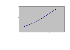
3.3 Heat Capacity
As explained in theory, the inverse of the slope of the dispersion curves leads to density-of-states which indicate how the energy is partitioned in various normal modes. These are shown in Fig. 2(b) and 3(b) respectively. The peaks in the frequency distribution curves compare well with the observed frequencies. The frequency distribution function can also be used to calculate the thermodynamical properties such as heat capacity, enthalpy changes etc. It has been used to obtain the heat capacity as a function of temperature. The predictive values of heat capacity have been calculated and plotted within temperature range 50-
500 K (Fig. 4)
Fig. 4 Variation of heat Capacity with temperature of PNIPAm.
It may be added here that the contribution from the lattice models is bound to make a difference to the heat capacity because of its sensitivity to low frequency modes. However we have solved the problem only for an isolated chain. The calculation of dispersion curves for a three dimensional system is extremely difficult. Inter-chain modes involving hindered translator and rotatory motion will appear and the total number of modes will depend on the contents of the unit cell. It would not only make the dimensionality of the problem prohibitive but also bring in an enormous number of interactions which are difficult to visualize and quantify. Thus it makes the problem somewhat intractable. The inter-chain interactions will contribute to lower
IJSER © 2015 http://www.ijser.org
International Journal of Scientific & Engineering Research, Volume 6, Issue 4, April-2015 1882
ISSN 2229-5518
frequencies. They are generally of the same order and magnitude as in the weak inter-chain interactions. Their introduction would, at best bring about crystal field splitting at the zone center and zone boundary depending on the symmetry dependent selection rules. However, the inter-chain assignments will remain by and large undisturbed. Thus in spite of several limitations involved in the calculation of specific heat, the present work does provide a good starting point for further basic studies on the dynamic and thermodynamic behavior of conducting polymers which go into well defined conformations. The present work goes beyond it and calculates the dispersion curves within the entire zone.
4 CONCLUSION
The vibrational dynamics of PNIPAm can be satisfactorily interpreted from the dispersion curve and dispersion profile of the normal modes of PNIPAm as obtained by Higg’s method for infinite system. Some of the internal symmetry dependent features such as attraction and exchange of character are also well understood.
REFERENCES
[1] Wu C & Wang X, Phys Rev Lett 80(18) (1998) 4092.
[2] von Recum H A & Kim S W, J Biomat Sci-Polym E 9(11) (1998) 1241.
[3] Lee E & von Recum H A, J Biomed Mater Res-A 93 (2010) 411. [4] Chung J E, Yokoyama M, Yamato M, et al, J Control Release
62 (1999) 115.
[5] Hu Yan & Kaoru Tsujii, Colloid Surface B 46 (2005) 142.
[6] Yoshida R, Uchida K, Kaneko Y, et al, Nature 374 (1995) 242.
[7] Bae Y H, Okano T, Hsu R & Kim S W, Makromol Chem-Rapid
8(10) (1987) 481.
[8] Sami M, Jihan A, Sawsan A S, et al, Int J Polym Anal Ch 15 (2010) 1.
[9] Bingjie S, Yinan L & Peiyi W, Appl Spectrosc 61(7) (2007) 765. [10] Yaron P, Ellina K, Lulu F, et al, J Polym Sci Pol Phys 42 (2004)
33.
[11] Zeeshan A, Edward A G, Konstantin V P, et al, J Phys Chem B
113(13) (2009) 4284.
[12] Tuncer C, Simin K, Gokhan D, et al, Polym Int 56 (2007) 275. [13] Boon M T, Stuart W P, Gareth J P, et al, J Phys Chem B 114(9)
(2001) 3178.
[14] Shao H S & Li J L, Chinese Chem Lett 17(3) (2006) 361.
[15] Wilson E B, Decuis J C & Cross P C, Molecular Vibrations: The Theory of Infrared and Raman Vibrational Spectra, (Dover Publications, New York), 1980.
[16] Higgs P W, Proc R Soc Lond 220 (1953) 472.
[17] Tondon P, Gupta V D, Prasad O, et al, J Polym Sci Pol Phys 35 (1997) 2281.
[18] Pan R, Verma M N & Wunderlich B, J Therm Annl 35 (1989)
955.
[19] Roles K A, Xenopoulos A & Wunderlich B, Biopolymers 33 (1993) 753.
[20] Bingjie S, Yinan L & Peiyi W, Appl Spectrosc 61(7) (2007) 765.
IJSER © 2015 http://www.ijser.org