Cellular Neural Networks
Like cellular automata, the CNN is made of a massive aggregate of regularly spaced circuits clones, called cells, which communicate with each other directly only through
Every cell is connected to other cells within a neighborhood of itself. In this scheme, information is only exchanged between neighbouring neurons and this local information characteristic does not prevent the capability of obtaining global processing. The CNN is a dynamical system operating in continuous or discrete time. A general form of the cell dynamical equations may be stated as follows:
nearest neighbors. In Figure 2, each cell is modeled as squares. The adjacent cells can interact directly with each
other. Cells not directly connected together may affect
d xij (t )
![]()
C
dt
= − xij (t) +
each other indirectly because of the propagation effects
∑
kl∈N r (ij )
kl
A(i−k )( j −l ) (t ) y
+ ∑
kl∈N r (ij )
B(i−k )( j −l ) (t )ukl + I
of the continuous-time dynamics of cellular neural
![]()
![]()
![]()
![]()
y (t ) = 1 (x (t ) + 1 − x (t ) − 1 )
networks. An example of a two-dimensional CNN is shown in Figure 3. Now let us define the neighborhood of C(i,j).
![]()
ij 2 ij ij
( 2 )
Definition : r-neighbourhood
The r-neighbourhood of a cell C(i,j) , in a cellular neural network is defined by,
where x,y,u,I denote respectively cell state, output, input, bias and j and k are cell indices. CNN parameter values are assumed to be spaced-invariant
and the nonlinear function is chosen as piece-wise
![]()
N r (i, j) = {C(k, l )}![]() max{
max{![]() k − i
k − i
1 ≤ k ≤ M ;1 ≤ l ≤ N
![]()
, l − j
}≤ r
}
(1)
linear. Since we use discrete 2-D images, Equation
(2) is rewritten as,
where r is a positive integer number.
xij (n + 1)
= − xij (n) +
Figure 3 shows neighborhoods of the C(i,j) cell (located at the center and shaded) with r=1 and 2,respectively. To
∑
kl∈N r (ij )
kl
A(i−k )( j −l ) (t )(n) y
+ ∑
kl∈N r (ij )
B(i−k )( j −l ) (t )ukl + I
show neighbourhood relations more clearly, the center
![]()
![]()
![]()
![]()
![]()
y (n) = 1 (x (n) + 1 − x (n) − 1)
(3)
pixel is coloured as black and related pixels in brown in
ij 2
ij ij
Figure 3 and 4. Cells are multiple input-single output nonlinear processors all described by one, or one among several different, parametric functionals. A cell is characterized by a state variable, that is generally not observable as such outside the cell itself. It contains linear and non-linear circuit elements such as linear resistors, capacitors and non-linear controlled sources (Figures 4 and 5).
with A, B and I being cloning template matrices that are identically repeated in the neighbourhood of every neuron as,
a−1,−1
A = a0,−1
a
1,−1
b−1,−1
b
B = b0,−1
1,−1
a−1,0 a0,0 a1,0
b−1,0 b0,0 a1,0
a−1,1 a0,−1 a−1,1
b−1,1
b0,−1 , I
b−1,1
(4)
image processing, motion detection, pattern recognition, simulation. The reduced number of connections within a local neighbourhood, the principle of cloning template etc., turn out to be advantage of CNN's.
The network behaviour of CNN depends on the initial state of the cells activation, namely bias I and on weights values of A and B matrices which are associated with the connections inside the well-defined neighbourhood of each cell. CNN's are arrays of locally and regularly interconnected neurons, or, cells, whose global functionality are defined by a small number of parameters (A,B, I) that specify the operation of the component cells as well as the connection weights between them. CNN can also be considered as a nonlinear convolution with the template. Cells can be characterized by a functional block diagram that is typical of neural network theory: Figure 4 depicts a two- stage functional block diagram of a cell, composed of a generalized weighted sum (in general nonlinear with memory) integration, output nonlinear function/functional. Data can be fed to the CNN through two different ports: initial conditions of the state and proper input u. Bias values I may be used as a third port. The network behaviour of CNN depends on the initial state of the cells activation, namely bias I and on weights values of A and B matrices which are associated with the connections inside the well-defined neighbourhood of each cell. CNN's are arrays of locally and regularly interconnected neurons, or, cells, whose global functionality are defined by a small number of parameters (A,B, I) that specify the operation of the component cells as well as the connection weights between them. CNN can also be considered as a nonlinear convolution with the template. Since the introduction of Chua [2], CNN has attracted a lot of attention. Not only from a theoretical point of view these systems have a number of attractive properties, but furthermore there are many well-known applications like
Behavioral Simulation
Recall that equation (1) is space invariant, which means that A(i,j;k,l) = A(i-k,j-1) and B(i,j;k,l) = B(i,k;,j,l) for all i,j,kl.
Therefore, the solution of the system of difference equations can be seen as a convolution process between the image and the CNN processors. The basic approach is to imagine a square subimage area centered at (x,y), with the subimage being the same size of the templates involved in the simulation. The center of this subimage is then moved from pixel to pixel starting, say, at the top left comer and applying the A and B templates at each location (x,y) to solve the differential equation. This procedure is repeated for each time step, for all the pixels. An instance of this image scanning-processing is referred to as an “iteration”. The processing stops when it is found that the states of all CNN processors have converged to steady-state values[2] and the outputs of its neighbor cells are saturated, e.g. they have a
+1 value.
This whole simulating approach is referred to as raster simulation. A simplified algorithm is presented below for this approach. The part where the integration is involved (i.e. calculation of the next state) is explained in the Numerical Integration Methods section.
In the following two subsections we will discuss genetic algorithms and edge detection by CNN and genetic algorithms.
Genetic Algorithms
In the estimation of A.B. and I matrices of CNN, we use genetic algorithms. Genetic algorithm is a learning algorithm based on the mechanism of natural selection and genetics, which have proved to be effective in a number of applications. It works with a binary coding of the parameter set, searches from a number of points of the parameter space. It uses only the cost function during the optimization, it need not derivatives of the cost function or other information. [11,12]. Processes of natural selection cause chromosomes that encode successful structures to reproduce more often than those that do not. In addition to reproduction, mutations may cause the chromosomes of children to be different from those of their biological parents, and crossing over processes create different chromosomes in children by changing the some parts of the parent chromosomes between each other. Like nature, genetic algorithms solve the problem of finding good chromosomes by manipulating in the chromosomes blindly without any knowledge about the problem they are solving.[12]. The underlying principles of GA were first published by Holland in1962, [13]. The mathematical framework was developed in the 1960s and is presented in his pioneering book in 1975 [14]. In optimization applications, they have been used in many diverse fields such as function optimization, image processing, the traveling salesperson problem, system identification and control. A high-level description of GA has been done by Davis in 1991 as follows. [15] Given a way or a method of encoding solutions of problem into the form of chromosomes and given an evaluation function that returns a measurement of the cost value of the following steps:
Step1: Initialize a population of chromosomes
Step2: Evaluate each chromosomes in the population. Step3: Create new chromosomes by mating current chromosomes; apply mutation and recombination as the parent chromosomes mate.
Step4: Delete members of the population to make room for new chromosomes.
Step5: Evaluate the new chromosomes and insert them into the population.
Step6: If the stopping criterion is satisfied, then stop and return the best chromosome; otherwise, go to step3
Edge detection by CNN and genetic algorithms
In this work, proper CNN templates are described to locate edge detection in image by using genetic algorithms. For this aim, CNN templates are designed so that they satisfy the stability. So, A and B templates are selected as symmetric. Because of selecting size of templates as 3*3, totally 11 template parameters are searched. One of these parameters is offset, five of them belongs the A matrix, and the other five parameters belongs the B matrix. Each parameter are encoded by 16 bits in chromosomes. So, the length of chromosomes has been selected as 176 bits. In training process, 72 chromosomes are constructed as initial population randomly. The number of population is kept constant as 72 during the algorithm. Mutation probability m p has been set % 1. Training process includes these steps as follows.
(i).Construct initial population; A matrix is constructed called as population matrix. Each row of the population matrix represents chromosomes. Because of selecting number of chromosomes is 72, there are 72 rows in population matrix. Number of columns of this matrix is 176, because there are 176 bits in each chromosome. At the beginning this matrix is constructed randomly.
(ii). Extract the CNN template: Chromosomes represents the binary codes of the elements of the CNN template A,B, I . In this step, each chromosomes are decoded the elements of the CNN
are computed in [-8,8] interval. Since each element is coded as 16 bits, each parameter can take 216 different value in [-8,8] interval. In each chromosomes first 11 bits represents first bits of the template elements. And second 11 bits of chromosomes represents the second bits of the template elements and so on. These elements are
S = A11, A12 , A13 , A21, A22 , B11, B12 , B13 B21 B22, I (5)
(iii). Evaluate cost function value for each chromosomes; In this step, an image which was selected as training image is given as input to CNN. Normally in this gray- level image, brightness varies in 0 (black) through 1(white) interval. To fit this image to CNN operation, brightness of the image is converted from [0,1] to [-1,1]. According the same rule, brightness of the CNN output image is converted from [-1,1] to [0,1].Then CNN works with templates belonging with first chromosome. After the CNN output appears as stable, cost function is computed between this output image and target image which we want to obtain. This process is repeated with template sets belongs each chromosomes in the population. Cost function has been selected in this study as follow
maximum fitness in the population is selected. The templates which has been extracted from this selected chromosomes are the most proper the templates which satisfy the task we wanted to realize.
(iv). Creating new generation; Before creating next generation, fitness values of the population are sorted by descendent order. And all of the fitness values are normalized related to the sum of the fitness values of the population. A random number r between 0 and 1 is generated. Then the first population member is selected whose normalized fitness, added to normalized fitnesses of the proceedings population members, is greater than or equal to r . This operation is repeated 72 times. So, the chromosomes whose fitness are bad are deleted from the population. This procedure mentioned above is called reproduction process in genetic algorithms. Reproduction process does not generate new chromosomes. It elect the best chromosomes in the population and increases the number of the chromosomes whose fitness values are relatively
M N greater than the others.
Cost( A, B, I ) =
∑∑ Pi, j
⊕ T i, j
(6).
i j After the reproduction 36 pairs of chromosomes are
where A,B, I represents CNN templates, m, n represents number of pixels of the image, P and T represent input
and target image, respectively, notation ⊕ represents
XOR operation between each elements of the P and T . After the finding the cost function, fitness function is evaluated for each chromosome according this rule; fitness(A, B, I ) = m* n - cost(A, B, I ) (7). Another definition has been defined for stopping criterion as follows;
stcriterion = 0.99 *m* n (8).
where m represents the number of rows of the image matrix and n represents the number of the columns of the image matrix. If the maximum fitness value of the chromosomes is greater than stop criterion, algorithms is stopped and the chromosome whose fitness value is the
selected as parents randomly. Two numbers s1, s2 between 1 and length of chromosomes,176 are generated. The bit strings between s1 and s2 are called crossover site. During the crossing over process, bit strings in crossover site in each pair of chromosomes are interchanged. Then two new chromosomes are created from a pair of old chromosomes. At the last, 72 new chromosomes which are called children are generated to build new population. Over these chromosomes, mutation operation is processed. Since mutation probability has been set to %1, 126 bits are selected randomly in the population and they are inverted. And the chromosome whose fitness value was the best before the reproduction process is added instead of
deleted a chromosome which randomly selected in the population that was obtained after the mutation process population to save the best chromosome. This new
population is the next generation population. After the obtaining the new generation searching procedure goes to second step and goes on until the stopping criterion was
happened in the second step.
This gives,
Where
B
ε ij =
i=3
∑
i=1
bi, j
+1 sign(u
i, j +!
) (9)
Time multiplexing simulation approach
bi, j +1 = The missing entries from the B template due to the absence of input signals u i, j+l
sign(.) = The sign
function
In this procedure it is possible to define a block of CNN processors which will process a subimage whose number of pixels is equal to the number of CNN processors in the block. The processing within this subimage follows the raster approach adapted in Chua and Yang (1988b). Once convergence is achieved, a new subimage is processed. The same approach is being carried out until the whole image has been scanned. It is clear that with this approach the hardware implementation becomes feasible since the number of CNN processors is finite. Also, the entire image is scanned only once since each block is allowed to fully converge. An important point is to be noticed that the processed border pixels in each subimage may have incorrect values since they are processed
The latter function is used to represent the status of a pixel, e.g. black = 1 and white = -1. It is seen that the error is both image and template dependent. Alternatively, the steady state of a border cell may converge to an incorrect value due to the absence of its neighbors weighted input. Given the local interconnectivity properties of CNN, one can conclude that the minimum width of the input belt of pixels is equal to the neighborhood radius of the CNN. Interaction between Cells in view of interaction between cells, it is possible to compute the absolute error in a similar way. In absence of the B template for a moment, the error is expressed as:
without neighboring information only local interactions are important for the latency of CNNs. To overcome the
aforementioned problem two sufficient conditions must
A
ε ij
i=3
= ∑bi, j +1 yi, j +1 (t)
i=1
(10)
be considered while performing time-multiplexing simulation. Alternatively, to ensure that each border cell properly interacts with its neighbors it is necessary to have the following. (1) To have a belt of pixels from the original image around the subimage and (2) to have pixel overlaps between adjacent subimages.
It is possible to quantize the processing error of any border cell Cij with neighborhood radius of 1. By computing independently the error owing to the feed forward operator and interaction among cells for the two horizontally adjacent processing blocks, the absoulte
Where
ai, j +1 = The missing entries from the A template due to the absence of input signals y i, j+l (t)
In this case output signals depend on the state of their corresponding cells. The technique of an overlap of pixels between two adjacent blocks is proposed in order to minimize the error. The minimum overlap width must be proportional to two times of the neighborhood`s radius of the CNN. The time-multiplexing procedure deals with iterating
each block (subimage) until all CNN cells within the block converge. The block with converged cells will have state variables x which are the values used for the final output image shown in Fig. 1, the converged values from Block i are taken by the left side of the overlapped cells and the right side from Blocki+1. Further, the initial conditions for the border cells of Block i+1 are the state values obtained while processing Block i-1. In the simulator used here, the number of overlapping columns or rows between the adjacent blocks is defined by the user. Suppose if higher number of overlapping is obtained in columns or rows then it indicates the more accurate simulation of neighboring effects on the border cells.
Fig. 1: CNN multiplexing with overlapped cells
In case of practical applications the correct final state is of more importance than the transient states, an overlap of two is usually sufficient. An even number of overlapping cells is recommended, because the converged cells in the overlapped region can be evenly divided by the two adjacent blocks. Having the added overlapping feature, better neighboring interactions are achieved, but at the same time, an increase in computation time is unavoidable. On the other hand, by taking advantage of the fact that the original input image is been divided into small CNN subimages, the chance of
a subimage having all its pixels black or white is high. This is another feature that can be added to the time multiplexing simulation to improve computation times. The savings in simulation time come from avoiding repetitive simulations of all- black and all-white subimages. The notion behind this timesaving scheme is that when the very first all-black/all-white block is encountered, after processing that block, the final states of the block are stored separately from the whole image. When subsequent all-black/all-white blocks are found, there is no need to simulate these blocks since the converged states are readily available in memory, which in turn leads to avoiding the most time consuming part of the simulation which is the numerical integration. The overall idea of this simulation approach is given below in the form of program fragment.
Program Fragment for Time-Multiplexing CNN Simulation To understand the overall concept of overlap and belt approaches and raster simulation, the simplified version of algorithm with simulated annealing is given:
Algorithm: (Time-Multiplexing CNN simulation with genetic algorithm)
Obtain the input image, initial conditions and templates from user;
/* M,N = # of rows/columns of the image */
/* apply genetic algorithm in section 3.1*/
/* Use the optimized parameters from the algorithm
*/
B= {Cij = 1,..., block_x and j = 1,..., block_y}P C S = set of border cells (lower left corner) overlap = number of cell overlaps;
belt = width of input belt M = number of rows of the image N = number of columns of the image
for (i=0; i < M; i += block_x - overlap)
for (j=0; j < N; j += block_y - overlap)
/* load initial conditions for the cells in the block except for those in the borders */
for (p=-belt; p < block._x + belt; p++) for (q=-belt; q < block_y + belt; q++) { xi+p, j+q (t)=
uij
The raster approach implies that each pixel is mapped onto a CNN processor. That is, we have an image processing function in the spatial domain that can be expressed as:
g(x,y) = T(f(x,y))
(9)
1
− 1
∀Ci+ pj +q ∈ B
where f(.) is the input image, g(.) the processed
image, and T is an operator on f(.) defined over the
}/* end for */
/* if the block is all white or black don't process it */
if (xi+ p j +q = −1 ∨ xi+ p j +q = 1∀Ci+ pj +q )
{
obtain the final states from memory; continue;
}
do { /* normal raster simulation */ for (p=O; p < block_x; p++) (
for (q=O; q < block_y; q++)
/* calculation of the next state excluding the belt of inputs
*/
xi+pj+q (tn+1) = xi+pj+q (tn+1) +
tn +1
∫ f ′(xi + p j + q (t n ))dt ∀Ci + pj +q ⊂ B
tn
/* convergence criteria */
neighborhood of (x,y).
Numerical Integration Methods
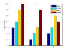
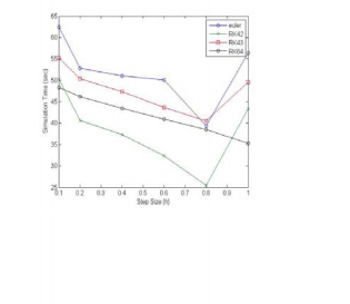
four of the single-step numerical integration algorithms used in the CNN behavioral simulator described here. They are Euler, RK4(2), RK4(3) and RK6(4).
The Proposed Methods
dx If
i + p, j +q (tn )

= 0 and y kl
dt
= ±1 c(k, l) ∈ N r
(i + p, j + q)
and RK6(4).
converged_cells++;
}/* end for */
/* update state values */ xi+pj+q (tn+1) = xi+pj+q (tn )
while(converged_cels < (block_x *block_y));
/* store new state values excluding the ones corresponding
Stepsize selection algorithm.
There are currently two widely used methods that
have appeared in the literature for changing the stepsize of p (q)-order RK codes. The first is to apply the formula (see [9])
to the border cells */
TOL ,
1
q+1
1
hn+1 = f
(10)
A ← xij ∀Cij ∈ B \ P
}/* end for */
EST n
Where f1 is a safety factor and the new sought-after stepsize hn+1 = xn+1 - xn is predicted in terms of an
estimate of the local error ESTn which is based on the approximation
^
five calculated derivates is given:

19

203
n n
EST n ≈ y − y ,
(11)
xij((n+1)τ) =xij(nτ) + 130
k1ij
+ 990
k2ij
^
Assuming yn , yn
to be the pth-, qth-order approximate
1331

+ 3159
73

k3ij + 486
k4ij (15)
solutions, respectively, at the previous grid point xn and TOL the requested tolerance. If
The difference between Rk4(2) and RK4(3) is the local truncation error in the case of RK4(2) is given
by using the RK(2)i.e.
EST n ≤ TOL,
(12)
Then the computed solution yn+1 is accepted and the integration is carried out, otherwise(5) is reevaluated by substituting
yij
((n+1)τ) =yij
13
4

(nτ) + 55
k1ij +
343

1215
k2ij
EST n → EST n +1
(13)

+ 18
k3ij (16)
This methodology is termed the error per step (EPS)
mode (see Shampine [10]).
An alternative is to consider the same algorithm (5), but to use, instead of (6), the approximation
But local truncation error in the case of RK4(3) is given by using the RK(3)i.e.
EST n ≅
∧
n
n
y − y

,
hn
(14)
yij((n+1)τ) =yij(nτ) +
11

130
k1ij +
637

1215
k2ij
This is called error per unit step (EPUS) [10].
RK4(2) and RK4(3) at n = 4
According to [8], The equations of RK4(2) and RK4(3) are:
k1ij = τf΄(xij (nτ))
605

+ 3159
k3ij -
73

1215
k4j (17)
5

k2ij = τf΄(xij (nτ))+ 14

52
k1ij

819
RK6(4) at n= 6
According to [8], The equations of RK6(4) are: k1ij = τf΄(xij (nτ))
k3ij = τf΄(xij (nτ))- 605
k1ij + 1210

k2ij 4
2576


k4ij = τf΄(xij (nτ))+ 4745 1089
252

k1ij - 365
k2ij +
k2ij = τf΄(xij (nτ)) + 27

1
k1ij

1
949
k3ij


19 343
k3ij = τf΄(xij (nτ)) + 18
66

k4ij = τf΄(xij (nτ))+ 343
k1ij + 6
727

k1ij - 1372
k2ij
k2ij +
k5ij = τf΄(xij(nτ))+ 130
k1ij + 1215
k2ij +
1053
1331
3159
73
k3ij + 486
k4ij

1372
k3ij
Therefore, the final integration is a weighted sum of the
13339
K5ij = τf΄(xij(nτ))+ 49152
4617
k1ij - 16384
k2ij +