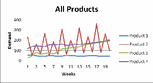
Figure 1: Historical Data for All Products
International Journal of Scientific & Engineering Research, Volume 5, Issue 5, May-2014 25
ISSN 2229-5518
Operations Planning & Control at Ross Product
Division
Ruwaid Arab
Index Terms— Cycle Times, Forecasting, Nutritionals, Process Analyzer, Scheduling, Simulation, Work In Progress.
—————————— ——————————
ur main objective is to perform a detail study on the Ross products with regards to its manufacturing process in various areas such as:
products which were insufficient to meet the upcoming de- mands of the customers, ultimately, resulted in drastic de- crease of the profits. This in turn led to customer dissatisfac- tion and decline of profits.
and higher cycle-time. By determining the root cause of the increase in (WIP) we would gradually decrease the average cycle-time and inventory cost.
tor in assigning jobs and recourses to various employees and placing them in proper shifts. It was due to the improper scheduling of the firm in the areas like not placing the em- ployees at the correct slots and inefficient methodology used for scheduling products resulted in off-putting effect on their overall performance.
Ross is planning to revise their production and planning strat- egy by hiring part time engineers to collect, analyze data and identify the best method for forecasting the demand, planning the production based on Bill of Materials (BOM).
The cost information of products and sub-products are collected as shown below on table 1:
Table 1: Cost Information of Products
IJSER © 2014
26
International Journal of Scientific & Engineering Research Volume 5, Issue 5, May-2014
ISSN 2229-5518
Table 2: Cost Information of Sub-Products
Sub- Product 1 | Sub- Product 2 | Sub- Product 3 | Sub- Product 4 | |
Regular Cost($/unit) | 23 | 22 | 12 | 9 |
Under-time cost | $2/min | |||
Buy M/c Cost | $2,500/machine | |||
Resale M/c Cost | $1,250/machine | |||
Constrains | No overtime or subcontracting allowed, Hold- ing cost based on ending inventory |
Forecasting is the method of predicting the company’s future sales demand. There are various approaches used in determin- ing the demand forecast namely,
Qualitative approach
Quantitative approach
If the company has a better understanding of the demand, it
can prove to be more significant and competitive in the worldwide market. The supplier needs to have the right amount of stock and this can be done only when there is enough knowledge of fluctuation of demand in the future. There is also a possibility of decrease in sales, when there in- sufficient supply of goods due to the underestimation of de- mand in the future. On the other hand when the demand is overestimated, this can lead to excess storage of stock result- ing in financial drain. The method that we used to build the forecasting models is as follows:
Table 3: Forecasting Methods for each Product
production plans to minimize cost and time:
Level Policy – Constant production rate throughout the year
Chase Policy – Producing exactly what is required
In our project we have made use of Material Requirements Planning (MRP) for all the products and sub-products based on the BOM (Bill OF Materials) to produce the forecasted de- mands.
Capacity planning is defined as process in which a company is able to withstand the required demand by having the neces- sary stock or inventory in hand at the right time. The main goal of capacity planning is to maximize the capacity of the company in terms of increase in efficiency and profitability and minimize the discrepancy such as factor affecting the ca- pacity planning namely ability of the workers, number of workers, production and suppliers. Aggregate planning is one of the popular methods of capacity planning it’s responsi- ble for matching the demand with the supply of goods thereby maintaining a tremendous production rates without backlogs.
Scheduling is crucial to the production planning process be- cause by performing scheduling properly a company can im- prove its efficiency and reduce its cost while maximizing its productivity.
Table 4: Demand Data
Product | Method |
Product 1 | Moving Average |
Product 2 | Seasonal Model With Trend Adjustment |
Product 3 | Linear Regression |
Product 4 | Exponential Smoothing |
The major concerns of production planning are to reduce the work in progress, determine the forecasting methods which are optimal and efficient, and finding the bottlenecks. When a firm is able to use their resources in an efficient way it means, that, they are performing well in their production planning department. A company plans its production either in long term, medium term or short term. Production planning in long term mainly focuses on increasing the capacity after various decisions taken by the firm. In case of medium term the com- pany mainly focuses on hiring or firing employees and mak- ing adjustments in increasing inventory.
The evaluation of products is carried out using two different
IJSER © 2014
27
International Journal of Scientific & Engineering Research Volume 5, Issue 5, May-2014
ISSN 2229-5518
Table 7: Production for the next 5 weeks
Figure 1: Historical Data for All Products
The first 10 weeks were used to forecast, and the recent 10 weeks were used to validate the forecast for the next 5 weeks.
Table 5: Forecast Summary
Weeks | Plan | |||||
21 | 22 | 23 | 24 | 25 | Plan | |
Product 1 | 47 | 47 | 47 | 47 | 47 | Level Plan Level Plan Chase Plan Chase Plan |
Product 2 | 253 | 253 | 253 | 253 | 253 | Level Plan Level Plan Chase Plan Chase Plan |
Product 3 | 204 | 213 | 221 | 229 | 238 | Level Plan Level Plan Chase Plan Chase Plan |
Product 4 | 202 | 208 | 213 | 218 | 224 | Level Plan Level Plan Chase Plan Chase Plan |
After calculating the MPS for each sub-product we started calculating the Capacity:
Table 8: Time Available in every Station
Table 9: # of Machines Required in every Station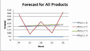
Figure 2: Forecast Summary
Level Policy and Chase Policy were used for our calculations:
Table 6: Production Plan for each Product
Table 10: # of M/C to Buy and Sell per week
Table 11: Total Cost of Machines
Total Cost | |||||
21 | 22 | 23 | 24 | 25 | |
Buy Ma- chine Cost | 125000 | 0 | 67500 | 0 | 2500 |
IJSER © 2014
28
International Journal of Scientific & Engineering Research Volume 5, Issue 5, May-2014
ISSN 2229-5518
Resale Ma- chine Cost | 0 | 46250 | 0 | 20000 | 2500 |
Cost For Each Week | $125,000 | $46,250 | $67,500 | $20,000 | $5,000 |
Total Cost | $263,750 |
We add more machines to minimize the total finish time and bring it below 40 hours. Using Process Analyzer Tool we changed the batch size and machine count to minimize the total processing time in order to minimize the total cost. The least utilized machines are removed to bring the total cost down.
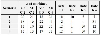
Table 12: Process Analyzer Output
Total Cost for each scenario is as follow:
Table 13: Total Cost for each Scenario
Scenario | Total Pro- cessing Time | Buy Machine Cost | Under Time Cost | Total Cost |
1 | Over 40 hours | --- | --- | --- |
2 | 29.05 | 90,000 | 87,481.2 | $177,481 |
3 | 33.22 | 90,000 | 58,576.82 | $ 148,577 |
4 | 35.03 | 80,000 | 20,503 | $100,503 |
Cycle times for each scenario are as follow:
Table 14: Cycle-times for each scenario
Cycle Time (min) | Avg. Cycle- Time (min) | |||
P1 | P2 | P3 | P4 | Avg. Cycle- Time (min) |
---- | ||||
1237.1 | 1021.23 | 1115.35 | 1750.34 | 1281.005 |
1423.72 | 1139.31 | 1141.46 | 1734.22 | 1359.67 |
1508.62 | 1368.43 | 1186.37 | 1973.05 | 1509.118 |
After the analysis and calculation, scenario four reflects the best result in terms of cost efficacy. On the other hand, scenar- io one will result in a shorter cycle-time but higher cost. The managers at Ross have to decide what will yield a higher cus- tomer satisfaction and will keep the company profitable.
IJSER © 2014