International Journal of Scientific & Engineering Research, Volume 5, Issue 2, February-2014 855

ISSN 2229-5518

Moving Obstacle Avoidance in Indoor

Environments

Ahmad Alsaab, Robert Bicker

Abstract— This paper deals with a problem of autonomous mobile robot navigation among dynamic obstacles. The velocity obstacle approach (VO) is considered an easy and simple method to detect the collision situation between two circular-shaped objects using the collision cone principle. The VO approach has two challenges when applied in indoor environments. The first challenge is that in the real world, not all obstacles have circular shapes. The second challenge is that the mobile robot cannot sometimes move to its goal because all its velocities to the goal are located within collision cones. For indoor environments some unobserved moving objects may appear suddenly in the robot path; particularly when the robot crosses a corridor or passes an open door. The contributions of this paper are that a method has been proposed to extract the collision cones of non-circular objects, where the obstacle size and the collision time are considered to weigh the velocities of the robot, and the virtual obstacle principle has been proposed to avoid unobserved moving objects. The experiments were conducted within indoor environments to validate the control algorithm proposed in this paper, and results obtained showed the mobile robot successfully avoided both static and dynamic obstacles.

Index Terms— Collision cone, Dynamic obstacle, Indoor navigations, Mobile robot, Non-circular object, Unobserved obstacles, Velocity obstacle approach.

1 INTRODUCTION

——————————  ——————————
utonomous ability of mobile robots provides large appli- cation areas including routine tasks such as office clean- ing and delivery, access to dangerous areas that are un-
reachable by humans such as cleanup of hazardous waste sites in nuclear power stations and planetary explorations. The key challenge of a mobile robot is to avoid obstacles which may prevent it from reaching its goal. Many algorithms have been suggested to solve this problem such as the potential field al- gorithm (PFA) and the vector field histogram method (VFH), however these methods do not consider the kinematic con- straints of the mobile robot such as limited velocities and ac- celerations [1], [2]. The Dynamic Window Approach (DWA) considers these constraints, where a suitable pair of rotation and linear speeds is chosen to avoid obstacles through a circu- lar path, but it needs relatively long time to define the free

ue between 1 and 0 . However, they have not considered the collision time. In [8], [9], the grown obstacle radius was modi- fied depending on the collision distance and collision time. This algorithm can be applied to avoid circular obstacles. For non-circular obstacles, the robot has to fit the sensor data into circles using a circle fitting method [10], [11], [12]. The optimal time horizon principle has been proposed in [13], where the smallest time horizon is used to define the collision course velocities. In the simulation test, they used circular obstacle and considered the obstacle's speed known, however in the real world the robot has to extract the shapes of the obstacle from sensor data, grow them using the robot radius and then extract the collision cones.
collision velocities [3]. All the previous mentioned algorithms are suitable for avoiding static obstacles. The linear velocity obstacle algorithm (VO) was proposed to avoid moving obsta-

Robot

𝑣𝑟

Collision cone

Safe path

Target
cles, where it defines the collision situation between two circu- lar objects moving with constant velocities [4]. The non-linear V-Obstacle method was introduced as an extension of the VO algorithm to avoid obstacles moving on arbitrary trajectories [5].
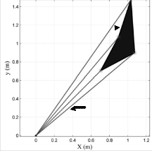
The first challenge of the VO algorithm is that in the real workspace, not all obstacles have circular shapes. The second challenge is that the mobile robot cannot sometimes move to its goal because all its velocities to the goal are located within collision cones as shown in Fig.1 , but there is at least one safe path to the goal. Many studies have been implemented the VO algorithm using simulation, furthermore they considered that obstacles have circle shapes and their velocities are known. For instance, [6] , [7] proposed the probabilistic collision cone principle, where the grown obstacle is extended by uncertain- ty in the exact radii of the obstacle and robot, the collision probability in the exact collision cone is given a value 1, while into the uncertain area the collision probability is given a val-
Grown obstacle

Fig. 1. The robot cannot reach its target according to the VO method

A mobile robot avoids dynamic obstacles by collecting in- formation about its surrounding environment using sensors. It then clusters the sensor data and utilizes a tracking algorithm to estimate the velocities and locations of obstacles. 2D scanning laser sensors are common in mobile robot applications, provide accurate information about the robot workspace, require a rela- tively small computation time and are unaffected by changes in illumination.
There are two types of laser data cluster methods; the dis- tance-based clustering methods [14], [15], [16] and kalman filter- based methods [17]. The KF-based methods detect the segments and their directions precisely, but are more complex than the distance-based methods and require relatively large computa-

IJSER © 2014 http://www.ijser.org

International Journal of Scientific & Engineering Research, Volume 5, Issue 2, February-2014 856

ISSN 2229-5518

tion time.
Some unobserved moving objects may appear suddenly in
the robot’s path; particularly when the robot crosses a corridor
the distance between the robot and the target.
The reference speed to the target is given as following:
𝑣𝑚𝑎𝑥 𝑖𝑖 𝑑𝑡 > 𝑑𝑡ℎ

(3)

or passes an open door. The robot must be able to anticipate
𝑣𝑡 = � 𝑣
𝑑𝑡
𝑜𝑜ℎ𝑒𝑒𝑒𝑖𝑒𝑒
such scenarios and manoeuvre to avoid collisions. The mobile
robot can define the opened doors and corridors by extracting
walls from the sensor data. There are many methods to extract walls from the laser data such as the Hough Transform Algo- rithm, line regression method, line tracking algorithm and itera- tive-end-point-fit algorithm [18], [19,] [20], [21], [22]. This paper
uses the Iterative-end-point-fit algorithm which is considered as a simple and robust method to extract lines from 2D laser sen- sors.
In this work, reactive control architecture was adopted, where a 2D laser sensor was utilized to recognize the robot's workspace and the laser data was clustered using the distance- based clustering method proposed in [16]. The extended parti- cle filter algorithm (EXPF) proposed in [23] was used to esti- mate the obstacle velocity. A method was demonstrated to ex- tract the collision cones of circular and non-circular objects. Fur- thermore, the collision time and the obstacle size were consid- ered. The virtual obstacle principle was proposed to avoid un- observed obstacles which may appear from opened doors.

2 REACTIVE CONTROL SYSTEM

Reactive control architecture was adopted in this study to produce the control command for the mobile robot as shown in Fig. 2, the sensor data comes from the laser sensor and odome- try data. In the first stage, the laser data is clustered into sepa- rate groups (obstacles) using the distance-based clustering method proposed in [16]. In the second stage, the obstacles ve- locities are estimated by a tracking algorithm using the extend- ed particle filter. While the third stage includes three behaviours namely Go to Goal, Obstacle Avoidance and Unobserved obsta- cle avoidance. In the fourth stage, the outputs of the behaviours are fused to produce the control commands.

𝑚𝑎𝑥 𝑑𝑡ℎ

where 𝑣𝑚𝑎𝑥 and 𝑑𝑡ℎ denote the robot's maximum speed and
threshold distance respectively.

2.2 Obstacle Avoidance behaviour

2.2.1 Collision Cone of non-circular Obstacle

The original velocity obstacle method supposes that the ro- bot and obstacle have circular shapes. The boundary of collision cone is defined by the two tangents of the grown obstacle circle and the centre of the robot as shown in Fig. 3. The left and right angles of the tangents are given as following:

𝑒

𝐿

where 𝑑 is the distance between the robot centre and the ob- stacle centre, 𝐿 is the tangent length, ∅ is the angle between the obstacle and the robot in the global frame, ∅𝑙 , ∅𝑟 are the left and right tangent angles, (𝑥𝑟 , 𝑦𝑟 ), (𝑥𝑜 , 𝑦𝑜 ) are the robot and
obstacle coordination.

2D laser

Odometry

Data

Go to Goal

Obstacle

Avoidance

Unobserved Obstacle Avoidance

Decision

Unit

Control

Comannds

Sensor data First Stage Second Stage Third Stage Forth Stage

Fig. 2. The proposed reactive control system

2.1 Go to Goal Behaviour

This behaviour utilizes the current robot position coming from the odometry sensors and the goal position to define the speed and direction to the target. In the global reference frame, the angle to and the distance between the robot and the target are given as:

where (𝑥𝑡 , 𝑦𝑡 ) and (𝑥𝑟 , 𝑦𝑟 ) represent the target and robot posi- tions with respect to the global reference frame. 𝑑𝑡 represents

Fig. 3. Velocity obstacle approach

Suppose there is a circular obstacle as shown Fig. 4, in which some points in the obstacle circumference were grown by the
robot radius rr. It can be noticed that the outer boundaries of the
grown points produced the grown obstacle circle. However, the
left and right tangent angles θli , θri of a grown point can be cal-
culated using equations [4],[5],[6], [7], [8]. The collision cone
boundaries of the obstacle are determined by the right tangent
which has the minimum angle and the left tangent which has
the maximum angle.
In this project a method is proposed to find the actual colli-
sion cone of a non-circular obstacle by the following steps:
• Each laser point is grown by robot radius.

IJSER © 2014

http://www.ijser.org

International Journal of Scientific & Engineering Research, Volume 5, Issue 2, February-2014 857

ISSN 2229-5518

• Calculating the left tangent angles 𝜃𝑙1 , , , 𝜃𝑙𝑛 and right tangent angles 𝜃𝑟1 , , , 𝜃𝑟𝑛 of the grown laser points,
where n refers to total number of laser points.
• Taking the maximum of the left tangent angles
𝜃𝑙1 , , , 𝜃𝑙𝑛 represents the left tangent angle of the
grown obstacle, and the minimum value of the right
tangent angles 𝜃𝑟1 , , , 𝜃𝑟𝑛 represent the right tangent
angle
requirement. The virtual obstacle principle has been proposed to avoid unobserved moving objects, in which a virtual circular obstacle is created at the start point of each open door threshold and corridor cross as shown in Fig. 5. The virtual radius is modified depending on the robot speed as the following equa- tion:
𝑒𝑜 = 𝑅. 𝑣𝑖 (13)
where 𝑅 is a constant positive value. 𝑣𝑖 represents the robot
speed

Mobile Robot

Wall

Virtual Obstacle

𝒓𝟎

Fig. 4. Growing the circumference points

2.2.2 Considering the collision time and obstacle size

The collision time and obstacle size are considered by assign- ing the robot velocities with different weights. Thus all free col-
lision velocities are given weights of numeric value 1, while the
weights of the collision course velocities are given as follows:

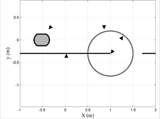
Fig. 5. The Virtual obstacle principle

The collision cone of the virtual obstacle is calculated depend- ing on the equations [3],[4],[5],[6], [7]. Likewise In this behav- iour, the robot velocities are weighed according the following:
1 𝑖𝑖 𝑑𝑟𝑜 > 𝑑𝑡ℎ
𝑊𝑢𝑛𝑜𝑏 = �exp �− 𝑡𝑢𝑛𝑜𝑏 � ∗ �1 − 𝑏
∗ 𝛿 ∗ 𝑜 (𝑖)� (14)

0 𝑖𝑖 𝑜𝑐 (𝑖) < 𝑜𝑐𝑡ℎ
(9)
𝑜𝑐 (𝑖)

𝑢𝑛𝑜𝑏 𝑐

𝑊𝑒𝑖 = �exp � −𝑡 � ∗ �1— 𝑏 ∗ 𝛿 ∗ 𝑜 (𝑖)� 𝑜𝑜ℎ𝑒𝑒𝑒𝑖𝑒𝑒
𝑡𝑢𝑛𝑜𝑏 , 𝑏𝑢𝑛𝑜𝑏and 𝑑𝑡ℎ are constants. 𝑑𝑟𝑜 refers to the distance

𝑜𝑐 (𝑖)

𝑐

𝛿 = min(∅𝑙 — 𝜃𝑖 , 𝜃𝑖 — ∅𝑟 ) (10)

between the robot and the door threshold.

2.4 Decision unit

where 𝑜𝑐 (𝑖) refers to the collision time. 𝑡, 𝑏 are constants, 𝑜𝑐𝑡ℎ
is the critical collision time, 𝜃𝑖 is the velocity angle.
The robot velocities within a collision cone have different
collision distances depending on the obstacle shape. However
the collision distance of the robot velocity (𝑣𝑖 , 𝜃𝑖 ) is given as:
where 𝑙𝑡𝑒𝑒𝑒𝑑𝑡𝑜𝑡, 𝐼 and 𝜎 refer to return laser points, index and the angle resolution of the laser sensor respectively. 𝑖𝑙𝑜𝑜𝑒 is a
function which gives the integral value.

2.3 Unobserved Obstacle Avoidance

The main task of this block is to fuse the outputs of the be- haviours and then generate the control commands which min- imize the collision risk and maximize the speed to the goal. The robot velocities are weighted depending on the output of the Go to Goal behaviour and the weights coming from the Obstacle Avoidance and Unobserved avoidance behaviours.
𝑒𝑖 = min(𝑊𝑢𝑛𝑜𝑏 , Ws) ∗ (𝛼1 + cos(𝜃𝑡 − 𝜃𝑖 )) ∗ (𝛼2
− ‖𝑣𝑡 − 𝑣𝑖 ‖) (15)
where 𝛼1 , 𝛼2 are constants.
The maximum weight velocity (𝑣𝑐 , 𝜃𝑐 ) is chosen to produce
control commands given as:
• The rotation speed is given as:
In indoor environments, some unobserved moving objects may appear suddenly in the robot path; particularly when the robot crosses a corridor or passes an open door. Therefore the
where 𝑘𝑤 is constant
𝜔𝑐
= 𝑘𝑤
. 𝜃𝑐
(16)
robot has to consider these obstacles and implement an action
to minimize the collision risk with the unobserved obstacles.
In this project a simple method was introduced to meet this

IJSER © 2014

• The linear speed is given as
http://www.ijser.org

International Journal of Scientific & Engineering Research, Volume 5, Issue 2, February-2014 858

ISSN 2229-5518

Obstacle
where 𝑘𝑣 is a constant, 𝑣𝑚𝑎𝑥 and 𝜔𝑚𝑎𝑥 represent the maximum
linear and rotation speeds of the mobile robot.

3 RESULTS AND DECISION

Experiments were implemented using two robots; the Pio- neer P3-DX robot and Nubot robot which was made in New- castle University. The experiments aimed to show that the robot can avoid collision with obstacles which have different intelli- gence levels, and minimize the collision risk with unobserved moving objects. Obstacles were classified according to the ob- stacle avoidance method into three classes; non-intelligent ob- stacles which do not have any obstacle avoidance algorithm, the low-level intelligent obstacles have ability to avoid static obsta- cle, and intelligent obstacles (Human).
The maximum linear and rotation speeds of the robots were
adjusted to 0.5 m/s and 100 degree/s respectively. In equation
[3], the threshold distance was chosen to be dth = 1 m. The pa-
rameters of the weighting fuction in equations [9], [14] for the
obstacle avoidance and unobserved obstacle avoidance behav-
iours were chosen to be a = aunob=5, b = bunob = 0.5. The con- stant value in equation [13] was chosen tobe 0.5m.the parame- ters a1 and a2 in equation [15] were assigned to the values 0.1 and 0.6 respectively. The parameters kw and kv were selected to
be 1 and respectively.

3.1 Collision Cone

The collision cone produced by the method demonstrated in this paper is compared with that produced by two fitting circle algorithms proposed in [11], [12]. Fig. 6 shows a virtual non- circular obstacle, in which the laser angle resolution was chosen to be 5º. The returned laser points are listed in Table 1.

TABLE 1

COLLECTED LASER POINTS

Fig. 7 shows the fitted circles; the circle C1 is produced by applying the method proposed in [11], while the circle C2 is produced by the method proposed [12]. Obviously the circle C1
is relatively huge which produces a huge collision cone. There-
fore the comparison was made between the collision cones pro-
duced by the circle C2 and the algorithm developed in this
study.
The calculated radius of the circle C2 was 0.36𝑚 which was grown by the robot radius0.5𝑚. As result the calculated angle
of the collision cone of the circle C2 was 70º. However it can be
seen from Fig. 8 that the collision cone does not touch any
point of the grown laser points.
Laser beam

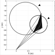
Fig. 6. Non-circular obstacle

C1
C2

Fig. 7. Fitted obstacle circles

For the proposed method, Table 2 lists the calculated tangent angles of each grown laser point, it can be noticed that the se- cond point has the maximum left angle and minimum right angle. Hence, it is not always correct to find the collision cone based on the first and last laser points of the laser cluster. The angle of the collision cone produced by the proposed method is
60º. Fig. 9 shows that the collision cone touches the grown ob- stacle at two points. Clearly the proposed method produced a collision cone which is more accurate and smaller than that produced by the circle fitting methods.

TABLE 2

COLLISION CONES FOR THE GROW N LASER POINTS

Grown obstacle

IJSER © 2014 http://www.ijser.org

International Journal of Scientific & Engineering Research, Volume 5, Issue 2, February-2014 859

ISSN 2229-5518

Grown laser point

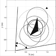
Fig. 8. Collision cone of the fitting circle

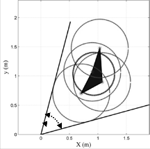
Fig. 9. Collision cone of the proposed method

3.2 Passing through a narrow Gap

The mobile robot (Pioneer P3-DX) had to pass through a nar- row gap as shown in Fig. 10. The robot's start point and target
were chosen to be (xr = 0m , yr = 0m) and (xt = 3m, xt = 0m) respectively, while the narrow gap was located at x = 1.55 m. The widths of the robot and narrow space were 0.45 m and
0.6 m respectively. Therefore the robot had free spaces of

75 mm at each side whilst passing through the narrow gap.

Fig. 10. The mobile robot has to pass the narrow gap

Fig. 11 shows that the robot was able to pass the narrow space without any collision. It can be seen that the robot imple- mented approximately a straight line during passing the nar- row space and then it turned to the goal in a curved path. On
hand Fig. 12 shows the robot speed vs. the x coordinate of the
mobile robot, in which the robot speed was increased form
0 m/s at x = 0 m to achieve the maximum speed of 0.5 m/s
atx = 0.6 m. When the robot became close to the gap at
x = 1.42 m it started to decrease, the speed became 0.34 m/s at
x = 1.57 m and then it increased after passing the narrow gap.
When the robot became close to its goal the speed was de-

creased gradually to become0 m/s.

Fig. 11. The mobile robot was able to pass the narrow gap

Fig. 12. The mobile robot speed

3.3 Avoiding a non-intelligent obstacle

The intelligent mobile robot (Pioneer robot) had to avoid a non-intelligent obstacle (Nubot Robot) Fig.13. The Nubot robot was not given any avoidance collision algorithm and moved
with a fixed speed0.5 m/s. The start positions of the robot and obstacle were chosen as (xr = 0m , yr = 0m) and (xt = 5m, xt =
0m) respectively. Fig.14. shows that The Pioneer robot was
able to avoid the non-intelligent obstacle without any collision.
It can be seen that the Pioneer robot moved on a straight line
from t = 0s till t= 3.6 s , and then avoided the moving obstacle, while at t = 7.5 s after the moving obstacle passed the robot
turned to its goal.

3.4 Avoiding a low-level intelligent moving obstacle

Here the Nubot robot having the ability to avoid static obsta- cles based on the potential field algorithm, where it used the laser data to produce the repulsive forces and the odometry data to produce the attractive force. The Pioneer started to avoid
the Nubot robot at t = 3 s as shown in Fig. 15. After the dynam-

IJSER © 2014 http://www.ijser.org

International Journal of Scientific & Engineering Research, Volume 5, Issue 2, February-2014 860

ISSN 2229-5518

ic obstacle passed the mobile robot turned to its goal (5m, 0 m)
at the moment t = 8 s. On other side the low-level intelligent
Nubot robot implemented a small avoidance manoeuvre there-
by avoiding the Pioneer robot at the momentt = 7 s. Clearly the
Pioneer robot started the avoidance manoeuvre 4 s before the
Nubot robot.

Fig. 13. The Nubot robot and Pioneer robot

Fig. 14. The robot avoided a non-intelligent obstacle

Fig. 15. The robot avoided a low-intelligent obstacle

3.5 Avoiding an intelligent moving obstacle

In this test, the robot had to avoid a human. As shown in Fig.
16 the robot turned to its right side at the moment t=3.74s to
avoid human, but also the human turned to the same direction
at the moment t=4s. Thus the robot turned right to avoid colli-

sion with human. The estimated of the human was 0.85 m/s.

Fig. 16. The robot avoided a human

3.4 Avoiding two dynamic obstacles

In this test, the robot had to avoid an obstacle moving in the same direction (Nubot) and an obstacle moving in the opposite direction (Human). The speed of the Nubot robot was adjusted as 0.35 m/s. As shown in Fig. 17, the human appeared in the laser data at the moment t=4s and disappeared at t=7s. On other side, the robot changed its direction to follow the moving obsta- cle (Nubot) and avoid the human at the moment t=4.8s, and after the human passed, the robot started to avoid the obstacle and reach its goal.

Fig. 17. The robot avoided an obstacle and human

4.5 Unobserved obstacle avoidance

The experiment workspace is shown in Fig. 18, in which the robot was located close to the wall. The robot had to reach its
goal (x = 6.5m, y = −3.3m) without causing colliding with any
obstacle. To avoid any causing damage to the robots, a simula-
tion test using Player/Stage simulator was carried out to show
that the robot may collide with an unobserved obstacle if it does not use the virtual obstacle principle. Fig. 19 shows the mobile robot collided with obstacle because the unobserved obstacle avoidance was removed from its control system.

IJSER © 2014 http://www.ijser.org

International Journal of Scientific & Engineering Research, Volume 5, Issue 2, February-2014 861

ISSN 2229-5518

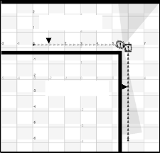
Fig. 18. The robot has to go to the goal and avoid an unobserved obstacle

Robot path

Obstacle path

Fig. 19. The mobile robot collided with the unobserved (simulation test)

Two real experiments were implemented for avoiding unob- served obstacles, Fig. 20 shows that the robot started to go away from the corner at the moment t=12s, while the dynamic obsta- cle appeared in the laser data at the moment t=17s, at the mo- ment t=18s the robot turned right to maximum the speed to its goal, but at the moment t=20s, the robot turned left again to avoid the collision with the dynamic obstacle. After the dynam- ic obstacle passed the robot returned to its goal.

Fig. 20. The mobile robot (Poineer) avoided the unobserved dynamic obstacle (Nubot)

In second test, the obstacle appeared in the laser data at the

moment t=15s as shown in Fig. 21. At the moment t=17s the robot reduced it speed and turned right to allow the moving obstacle to pass without any collision, after the collision risk with moving obstacle disappeared at the moment t=21s the ro- bot started to increase it speed and turn to its goal.

Fig. 21. The mobile robot (Pioneer) waited the unobserved dynamic ob- stacle (Nubot) to pass

4 CONCLUSION

In this paper, reactive control architecture has been adopted for mobile robot navigation in indoor environments. A simple method has been proposed to find the collision cones of circular and non-circular obstacles using a laser sensor, in which each laser point was grown by the robot radius, where the maximum left tangent represented the left boundary of the collision cone of the grown obstacle, and the minimum right tangent repre- sented the right boundary of the collision cone. The result has showed that the collision cone produced by the proposed meth- od is more accurate and smaller if compared with that pro- duced by the circle fitting methods. The collision time and the obstacle size were also considered to weigh the robot velocities.
The virtual obstacle principle has been proposed to avoid unobserved moving objects may appear suddenly form open doors, where a virtual circular obstacle is created at the start point of each door or corridor cross. The simulation test showed that the robot collided with an unobserved obstacle because the unobserved obstacle avoidance behaviour was removed from the control system, while the experiments showed that the robot was able to avoid unobserved obstacle appearing from corridor cross when the robot used the unobserved obstacle behaviour. Finally almost of the experiments have been captured and post- ed in the following website: https://www.facebook.com/pages/Robotics- Group/173949736063997

REFERENCES

[1] O. Khatib, “Real-time obstacle avoidance for manipulators and mobile ro- bots,” in in Robotics and Automation. Proceedings. 1985 IEEE International Conference, 1985, pp. 500–505.

IJSER © 2014 http://www.ijser.org

International Journal of Scientific & Engineering Research, Volume 5, Issue 2, February-2014 862

ISSN 2229-5518

[2] J. Borenstein and Y. Koren, “The vector field histogram-fast obstacle avoidance for mobile robots,” in Robotics and Automation, IEEE Transactions on, vol. 7, 1991, pp. 278–288.

[3] D. Fox, W. Burgard, and S. Thrun, “The dynamic window approach to collision avoidance,” in Robotics and Automation Magazine, IEEE, vol. 4, 1997, pp. 23–33.

[4] P. Fiorini and Z. Shiller, “Motion planning in dynamic environments using velocity obstacles,” in International Journal of Robotics Re- search, vol. 7, 1998, pp. 760–772.

[5] Large, Frederic, Laugier, Christian, and Z. Shiller, “Navigation among moving obstacles using the nlvo: Principles and applications to intelligent vehicles,” in Autonomous Robots, vol. 19, 2005, pp.

159–171.

[6] B. Kluge, “Recursive agent modeling with probabilistic velocity ob- stacles for mobile robot navigation among humans,” in in Intelligent Robots and Systems, 2003. (IROS 2003). Proceedings. 2003 IEEE/RSJ International Conference on, vol. 1, 2003, pp. 376–380.

[7] B. Kluge and E. Prassler, “Reflective navigation: individual behaviors and group behaviors,” in in Robotics and Automation, 2004. Proceed- ings. ICRA ’04. 2004 IEEE International Conference on, vol. 4, 2004, pp. 4172–4177.

[8] Z. Xunyu, P. Xiafu, and Z. Jiehua, “Dynamic collision avoidance of mobile robot based on velocity obstacles,” in in Transportation, Me- chanical, and Electrical Engineering (TMEE), 2011 International Con- ference on, 2011, pp. 2410–2413.

[9] M. Yamamoto, M. Shimada, and A. Mohr, “Online navigation of mobile robot under the existence of dynamically moving multiple obstacles,” in in Assembly and Task Planning, 2001,

[10] [ J. Guivant, E. Nebot, and H. Durrant-Whyte, “Simultaneous locali- zation and map building using natural features in outdoor environ- ments,” in Intelligent Autonomous Systems VI, 2000, pp. 581–588.

[11] W. Gander, G. H. Golub, and R. Strebel, “Least squares fitting of

circles and ellipses,” in BIT, vol. 34, 1994, pp. 558–875.

[12] J. Vandorpe, H. V. Brussel, and H. Xul, “Exact dynamic map build- ing for a mobile robot using geometrical primitives produced by a 2d range finder,” in in Robotics and Automation, 1996. Proceedings.,

1996 IEEE International Conference on, vol. 1, 1996, pp. 901–908.

[13] Z. Shiller, O. Gal, and T. Fraichard, “The nonlinear velocity obstacle revisited: the optimal time horizon,” in Workshop on Guaranteeing Safe Navigation in Dynamic Environments, the 2010 IEEE Int. Conf. on Robotics and Automation, Anchorage, AK (US), 2010.

[14] K. J. Lee, “Reactive navigation for an outdoor autonomous,” in in

Mechanical and Mechatroinc Engineering vol. Master: University of

Sydney, 2001.

[15] [K. Dietmayer, J. Sparbert, and D. Streller, “Model based object classi- fication and object tracking in traffic scenes from range images,” in In Proceedings of intelligent Vehicles Symposium, 2001.

[16] S. Santos, F. S. J.E. Faria and, R. Araujo, and U. Nunes, “Tracking of

multi-obstacles with laser range data for autonomous vehicles,” in in

3rd National Festival of Robotics Scientific Meeting (ROBOTICA)

Lisbon, Portugal, 2003, pp. 59–65.

[17] K. Rebai, A. Benabderrahmane, O. Azouaoui, and N. Ouadah, “Mov- ing obstacles detection and tracking with laser range finder,” in in Advanced Robotics, 2009. ICAR 2009. International Conference onl,

2009, pp. 1– 6.

[18] H. Koshimizu, K. Murakami, M. Numada, Global feature extraction

us- ing ecient hough transform, in: in Industrial Applications of Ma- chine Intelligence and Vision, 1989, pp. 298303.

[19] D. Dagao, M. Q. X. Meng, H. Zhongming, W. Yueliang, An improved hough transform for line detection, in: in Computer Application and System Mod- eling (ICCASM), 2010 International Conference on,

2010, pp. 354357.

[20] K. O. A. a. R. Y. Siegwart, Feature extraction and scene interpretation for map-based navigation and map building, in: in Proc. of SPIE, Mobile Robotics XII, 1997.

[21] V. Nguyen, A. Martinelli, N. Tomatis, R. Siegwart, A comparison of

line extraction algorithms using 2d laser rangender for indoor mobile robotics, in: in Intelligent Robots and Systems, 2005. (IROS 2005).

2005 IEEE/RSJ International Conference on, 2005, pp. 19291934.

[22] A. S. a. A. K. a. S. K. a. M. D. a. R. HUSSON, An optimized segmen-

tation method for a 2d laser-scanner applied to mobile robot naviga-

tion, in: in In Proceedings of the 3rd IFAC Symposium on Intelligent

Components and Instruments for Control Applications, 1997.

[23] M. M. Romera, M. A. S. VÃa˛zquez, and J. C. G. Garcà a, “Tracking multiple and dynamic objects with an extended particle filter and an adapted k-means clustering algorithm,” in Preprints of the 5th IFAC/EURON

IJSER © 2014 http://www.ijser.org