International Journal of Scientific & Engineering Research, Volume 5, Issue 2, February-2014 772

ISSN 2229-5518

Medical Image Fusion Based on Wavelet

Transform

Hari Om Shankar Mishra, Smriti Bhatnagar, Amit Shukla, Amit Tiwari

Abstract- The objective of Image fusion is to combine information from multiple images of the same scene in to a single image retaining the important and required features from each of the original image. Nowadays, with the rapid development in high-technology and modern instrumentations, medical imaging has become a vital component of a large number of applications, including diagnosis, research, and treatment. Medical image fusion has been used to derive useful information from multimodality medical image data. For medical diagnosis, Computed Tomography (CT) provides the best information on denser tissue with less distortion. Magnetic Resonance Image (MRI) provides better information on soft tissue with more distortion [1]. In this case, only one kind of image may not be sufficient to provide accurate clinical requirements for the physicians. Therefore, the fusion of the multimodal medical images is necessary [3]. This paper aims to demonstrate the application of wavelet transformation to multimodality medical image fusion. This work covers the selection of wavelet function, the use of wavelet based fusion algorithms on medical image fusion of CT and MRI, implementation of fusion rules and the fusion image quality evaluation. The fusion performance is evaluated on the basis of the root mean square error (RMSE) and peak signal to noise ratio (PSNR).

Index Terms - Medical Image Fusion, Computed Tomography(CT), Magnetic Resonance Image(MRI), Root mean square error (RMSE), Peak signal to noise ratio (PSNR), Multimodality images, Discrete wavelet Transform(DWT).

——————————  ——————————

1 INTRODUCTION

The term fusion means in general an approach to extraction of information acquired in several domains. The objective of Image fusion is to combine information from multiple images of the same scene in to a single image retaining the important and required features from each of the original image. The main task of image fusion is integrating complementary information from multiple images in to single image [6]. The resultant fused image will be more informative and complete than any of the input image and is more suitable for human visual and machine perception. Image fusion is the process that combines information from multiple images of the same scene. The object of the image fusion is to retain the most desirable characteristics of each image. Thus the new image contains a more accurate description of the scene than any of the individual image. It also reduces the storage cost by storing just the single fused image instead of multiple images. For medical image fusion, the fusion of image provides additional clinical information which is otherwise not apparent in the separate images. However, the instruments are not capable of providing such information either by design or because of observational constraints, one possible solution for this is image fusion.
Medical image fusion is the technology that could compound two mutual images in to one according to certain rules to achieve clear visual effect. By observing medical fusion image, doctor could easily confirm the position of illness. Medical imaging provides a variety of modes of image information for clinical diagnosis, such as CT, X-ray, DSA, MRI, PET, SPECT etc. Different medical images have different characteristics, which can provide structural information of different organs. For example, CT (Computed tomography) and MRI (Magnetic resonance image)
with high spatial resolution can provide anatomical structure information of organs. And PET (Positive electron tomography) and SPECT (Emission computed tomography) with relatively poor spatial resolution, but provides information on organ metabolism [3] [6]. Thus, a variety of imaging for the same organ, they are contradictory, but complementary and interconnected. Therefore the appropriate image fusion of different features becomes urgent requirement for clinical diagnosis.
Doctors can annually combine the CT and MRI medical images of a patient with a tumor to make a more accurate diagnosis, but it is inconvenient and tedious to finish this job. And more importantly, using the same images, doctors with different experiences make inconsistent decisions. Thus, it is necessary to develop the efficiently automatic image fusion system to decrease doctor’s workload and improve the consistence of diagnosis. Image fusion has wide application domain in Medicinal diagnosis.
In this paper, a novel approach for the fusion of computed tomography (CT) and magnetic resonance images (MR) images based on wavelet transform has been presented. Different fusion rules are then performed on the wavelet coefficients of low and high frequency portions [12]. The registered computer tomography (CT) and magnetic resonance imaging (MRI) images of the same people and same spatial parts have been used for the analysis.

II. IMAGE FUSION BASED ON WAVELET TRANSFORM

(A) WAVELET TRANSFORM

International Journal of Scientific & Engineering Research, Volume 5, Issue 2, February-2014 773

ISSN 2229-5518

Wavelet theory is an extension of Fourier theory in many aspects
Which is the sum over all time of signal

f (t )

multiplied by a
and it is introduced as an alternative to the short-time Fourier
transform (STFT). In Fourier theory, the signal is decomposed into sines and cosines but in wavelets the signal is projected on a set of wavelet functions. Fourier transform would provide good resolution in frequency domain and wavelet would provide good resolution in both time and frequency domains. The wavelet that provides a multi-resolution decomposition of an image in a biorthogonal basis and results in a non-redundant image representation. The basis is called wavelets and these are functions generated by translation and dilation of mother wavelet. In Fourier analysis the signal is decomposed into sine waves of different frequencies. In wavelet analysis the signal is
complex exponential (complex exponential can be broken down in to real and imaginary sinusoidal components).
The results of the transform are the Fourier Co- efficient F (ω) , which when multiplied by a sinusoidal of frequency ω , yields the constituent sinusoidal components of the original signals.
Similarly, the continuous wavelet transform (CWT) is defined as the sum over all time of the signal multiplied by scale, shifted version of the wavelet function

∞

decomposed into scaled (dilated or expanded) and shifted (translated) versions of the chosen mother wavelet or function. A wavelet as its name implies is a small wave that grows and decays

ψ C (scale, position) =

∫ f (t )ψ (scale, position, t )dt

− ∞

essentially in a limited time period [2] [8].
Wavelets were first introduced in seismology to provide a time dimension to seismic analysis that Fourier analysis lacked. Fourier analysis is ideal for studying stationary data (data whose statistical properties are invariant over time) but is not well suited for studying data with transient events that cannot be statistically predicted from the data’s past. Wavelets were designed with such
non-stationary data.
The results of the CWT are many wavelet co-efficient C, which
are a function of scale and position.
Multiplying each co-efficient by the appropriately scaled and shifted wavelet yields the constituent wavelets of the original signals.
We denote a wavelet as

“Wavelet transforms allow time – frequency localization”

Wavelet means “small wave” so wavelet analysis is about

ψ a ,b(t ) =

1 ψ ((t − b) / a)

(4)
analyzing signal with short duration finite energy functions.
They transform the signal under investigation in to another representation which presents the signal in a more useful form.
A wavelet to be a small wave, it has to satisfy two basic properties:
Where b=is location parameter
a=is scaling parameter
For a given scaling parameter a, we translate the wavelet by varying the parameter b. we define the wavelet transform as
(i) Time integral must be zero

∞

∫ψ (t )dt = 0

(1)

w(a, b) = ∫ t

f (t )

1 ψ ((t − b) / a)

(5)

− ∞

(ii) Square of wavelet integrated over time is unity

∞

∫ψ 2 (t )dt = 1

− ∞

Wavelet transform are two types
(2)
According equation (4), for every (a, b), we have a wavelet
transform co-efficient, representing how much the scaled wavelet
is similar to the function at location, t = b/a. [18]
“If scale and position is varied very smoothly, then transform is called continuous wavelet transform.”
Calculating wavelet co-efficient at every possible scale is a fair amount of work, and it generates an awful lot of data. What if we choose only a subset of scales and position at which to make our calculation. If we choose scales and position based on power

(a) CONTINUOUS WAVELET TRANSFORM (CWT)

Mathematically – the process of Fourier analysis is represented by the Fourier transform
of two so called dyadic scales and position then our analysis will
be much more efficient and just as accurate. We obtain such an analysis from the discrete wavelet transform (DWT).

F (ω) =

∞

∫ f (t )− jωt dt

− ∞

(3)

(b) DISCRETE WAVELET TRANSFORM (DWT)

An efficient way to implement (DWT) is- using filters. The DWT of a signal is calculated by passing it through a series of filters. First the signal is passed through a low pass filter and high pass

International Journal of Scientific & Engineering Research, Volume 5, Issue 2, February-2014 774

ISSN 2229-5518

filter. The outputs give the detail coefficients (from the high-pass filter) and approximation coefficients (from the low-pass).This
details of various sizes by projecting it onto the corresponding spaces. Therefore, to find such decomposition explicitly,
decomposition is repeated to further increase the frequency resolution.
additional coefficients

am, n

are required at each scale. At each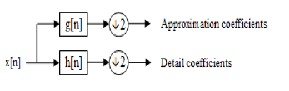

scale am, n

and

a m −1, n describe the approximations of the

function f (t) at resolution 2m and at the coarser resolution 2m −1 , respectively, while the co-efficient C m,n describe the information loss when going from one approximation to another. In order to

obtain the co-efficient C m,n

and am, n at each scale and position,

Figure 1: single level decomposition
a scaling function is needed that is similarly defined to equation (7). The approximation coefficients and the wavelet coefficients can be obtained: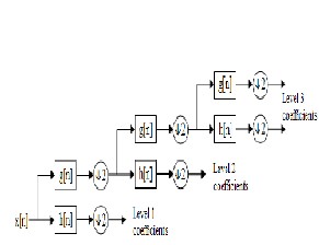

am, n = ∑ h2 n − k 2

(n − k )

am −1.k

(9)

C m, n =

∑ g 2 n − k 2

(n − k )

am −1, k

(10)
Where,

hn is a low pass FIR filter and

g n is related high pass

FIR filter. To reconstruct the original signal the analysis filters can be selected from a biorthogonal set which have a related set

of synthesis filters. These synthesis filters h
and g~ can be used
to perfectly reconstruct the signal using the reconstruction formula:

~ ~

Figure 2 : multilevel decomposition

am −1,l ( f ) = ∑[h 2 n − l am, n ( f ) + g 2 n − l C m, n ( f )]

(11)
Suppose that a discrete signal is represented by f (t); the wavelet decomposition is then defined as
Equations (9) and (10) are implemented by filtering and down sampling. Conversely eqn. (11) is implemented by an initial up sampling and a subsequent filtering [12].

f (t ) = ∑C m, n ψ m.n(t )

m, n

(6)
In a 2-D DWT, a 1-D DWT is first performed on the rows and then columns of the data by separately filtering and downsampling. These results in one set of approximation

−

where,ψ m, n(t ) = 2

2 ψ [2− m

t − n] and m and n are integers.

coefficients

I a and three sets of detail coefficients, as shown in

There exist very special choices of ψ such thatψ m, n(t )
Figure (3a), where I b ,

I c I d represent the horizontal, vertical

constitutes an orthogonal basis, so that the wavelet transform coefficients can be obtained by an inner calculation:
and dialog directions of the image I , respectively. In the language of filter theory, these four sub images correspond to the outputs of low–low (LL), low–high (LH), high–low (HL), and

C m, n = ( f ,ψ m, n) = ∫ψ m, n(t ) f (t )dt

(7)
high–high (HH) bands. By recursively applying the same scheme to the LL sub band a multiresolution decomposition with a desires level can then be achieved. Therefore, a DWT with
In order to develop a multiresolution analysis, a scaling function

ϕ is needed, together with the dilated and translated version of

K decomposition levels will have

M = 3 * K + 1 such

it,

 m 

frequency bands. Fig.1 (b) shows the 2-D structures of the
wavelet transform with two decomposition levels. It should be
noted that for a transform with K levels of decomposition, there

−  

is always only one low frequency band (LLk in figure (3b)), the

ϕ m, n

(t ) =2  2 ϕ[2− m t − n]

(8)
rest of bands are high frequency bands in a given decomposition level.
According to the characteristics of the scale spaces spanned by ϕ
andψ , the signal f (t) can be decomposed in its coarse part and
Structures of 2-D DWT:

International Journal of Scientific & Engineering Research, Volume 5, Issue 2, February-2014 775

ISSN 2229-5518

Figure 3(a): one stage of 2-D DWT multiresolution image decomposition

Figure 3(b): 2-D DWT structure with labeled sub bands in two- level decomposition [18].

III IMAGE FUSION METHOD

Image fusion method can be generally grouped in to three categories-
(i) Pixel level (ii) feature level (iii) decision level
Figure 4 : Level classification of the various popular image fusion methods based on the computation source.

(1) PIXEL LEVEL

Pixel level fusion is carried out on a pixel-by-pixel basis.

(2) FEATURE LEVEL

Feature level fusion requires an extraction of objects recognized in the various data sources. It operates on the salient features of the image such as size, shape, edge, pixel intensities or textures. These similar features from input images are fused.

(3) DECISION LEVEL

Decision-level fusion consists of integrating information at a higher level of abstraction, combines the results from multiple algorithms to yield a final fused decision. To extract information, input images are processed. The obtained information is then combined applying decision rules to reinforce common interpretation. Decision level fusion which deals with symbolic representation of images.
Pixel level fusion has the advantage that the images used contain the original measured quantities, and the algorithms are computationally efficient and easy to implement, the most image fusion applications employ pixel level based methods. Therefore, in this paper, we are still concerned about pixel level fusion [14].
Fusion methods are

(A) AVERAGE METHOD

In this method the resultant fused image is obtained by taking the average intensity of corresponding pixels from both the input image.
F (x, y) = (A (x, y) +B (x, y))/2
Where A (x, y), B (x, y) are input image and F (x, y) is fused image. And point (x, y) is the pixel value.
For weighted average method-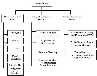

m n

F ( x, y) = ∑ ∑ (WA( x, y) + (1 − W )B( x, y))

x = 0 y = 0

(12)
Where W is weight factor and point (x, y) is the pixel value.

(B) SELECT MAXIMUM

In this method, the resultant fused image is obtained by selecting the maximum intensity of corresponding pixels from both the input image.

m n

F (x, y ) = ∑ ∑ Max(A(x, y ) + B(x, y ))

x = 0 y = 0

(13)

International Journal of Scientific & Engineering Research, Volume 5, Issue 2, February-2014 776

ISSN 2229-5518

Where A (x, y), B (x, y) are input image and F (x, y) is fused image, and point (x, y) is the pixel value.

(C) SELECT MINIMUM

In this method, the resultant fused image is obtained by selecting the minimum intensity of corresponding pixels from both the input image
3- The decision map is formulated based on the fusion rules.
4- The resulting fused transform is reconstructed to fused image by inverse wavelet transformation.

V. PERFORMANCE MEASURE PARAMETER

The two parameters used in my project to compare the fusion

m n

F ( x, y) = ∑ ∑ Min((A( x, y ) + B( x, y))

x = 0 y = 0

(14)
result.
1-The root mean square error (RMSE)
Where A (x, y), B (x, y) are input image and F (x, y) is fused image, and point (x, y) is the pixel value.

IV. IMAGE FUSION BY WAVELET

2-The peak signal to noise ratio (PSNR)
Let P (i, j) is the original image, F (i, j) is the fused image, (i, j) is the pixel row and column index and M and N are the dimension of the image. Then –
1-The root mean square error (RMSE) is given by-

M N 2

RMSE =

∑ ∑[P (i , j )− F (i , j )]

i=1 j =1

M × N

(15)

The smaller the value of the RMSE, the better the fusion performance [12].
2-The peak signal to noise ratio (PSNR) is given by-

PSNR = 10 × log

 ( f

2 max



RMSE 2 

(16)

10  

Where fmax is the maximum gray scale value of the pixels in the fused image. The higher the value of the PSNR, the better the fusion performance [16].
Figure (5) the image fusion scheme using the wavelet transforms.
A wavelet transform is applied to the image resulting in a four- component image: a low-resolution approximation component (LL) and three images of horizontal (HL), vertical (LH), and diagonal (HH) wavelet coefficients which contain information of local spatial detail. The low resolution component is then replaced by a selected band of the multispectral image. This process is repeated for each band until all bands are transformed. A reverse wavelet transform is applied to the fused components to create the fused multispectral image. Image fusion method is shown in above figure (5) [21].
The following steps are performed
1- The source images I1 and I2 are decomposed into discrete wavelet.
2-The decomposition coefficients: LL (approximations), LH, HL
and HH (details) at each level before fusion rules are applied.

VI. EXPERIMENTAL RESULTS

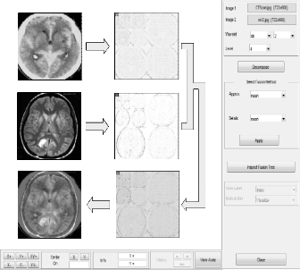
We considered five wavelet families namely Haar, Daubechies (db), Symlets, Coiflets and Biorsplines for fusing CT and MRI medical images. The filter -Daubechies (db) which produced the smallest RMSE was chosen for further analysis. Different fusion rules were tested, including the mean rule, maximum rule, and minimum rule. Here average rule gives better result, so average rule is selected. Here we applied average fusion rule to CT and MRI images. Figure 8(a) and 7(b) shows the resultant fusion of CT and MRI images.

International Journal of Scientific & Engineering Research, Volume 5, Issue 2, February-2014 777

ISSN 2229-5518

Image 1

Image 2

dwt

idwt

Decomposition 1

Decomposition 2

Synthesized Image

Fusion of Decompositions

Figure 6 : MRI and CT image fusion using matlab tool.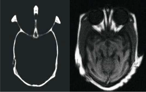

Figure 7 (a) : CT image (Brain) (b) MRI image (Brain)
Table -1
Table -2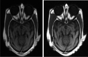

Figure 8 (a) : by average method (b) by maximum Method

VII. CONCLUSION

We have combined the wavelet transform and various fusion rules to fuse CT and MRI images. This method gives encouraging results in terms of smaller RMSE and higher PSNR values. Among all the fusion rules, the maximum fusion rule performs better as it achieved least MSE and highest PSNR values. Using this method we have fused other head and abdomen images. The

International Journal of Scientific & Engineering Research, Volume 5, Issue 2, February-2014 778

ISSN 2229-5518

images used here are grayscale CT and MRI images. However, the images of other modalities (like PET, SPECT, X-ray etc) with
their true color nature may also be fused using the same method.

REFERENCES

[1] Yong Yang, Dong Sun Park, and Shuying Huang, “Medical
Image Fusion via an Effective Wavelet based Approach”.
[2] S. S. Bedi, Rati Khandelwal, “Comprehensive and Comparative Study of Image Fusion Techniques” International Journal of Soft Computing and Engineering (IJSCE) ISSN: 2231-
2307, Volume-3, Issue-1, March 2013.
[3] F. E. Ali, I. M. El-Dokany, A. A. Saad, and F. E. Abd El- Samie, “Fusion of MR and CT Images Using The Curvelet Transform” 25th national radio science conference (nrsc 2008)
March 18‐20, 2008, Faculty of Engineering, Tanta Univ., Egypt.
[4] Mrs. Jyoti S. Kulkarni, “Wavelet Transform Applications”
IEEE 978-1-4244-8679-3/11/2011
[5] A. Soma Sekhar, Dr.M.N.Giri Prasad, “A Novel Approach of Image Fusion on MR and CT Images Using Wavelet Transforms” IEEE 2011
[6] Y. Zhang, “Understanding image fusion,” Photogramm. Eng. Remote Sens., vol. 70, no. 6, pp. 657–661, Jun. 2004.
[7] Krista Amolins, Yun Zhang, and Peter Dare, “Wavelet based image fusion techniques—an introduction, review and comparison”, ISPRS Journal of Photogrammetric and Remote Sensing, Vol. 62, pp. 249-263, 2007
[8] Li, H., B.S. Manjunath, and S.K. Mitra, 1995. “Multisensor image fusion using the wavelet transforms”, Graphical Models and Image Processing, 57:234–245.
[9] Jan Flusser, Filip ˇSroubek, and Barbara Zitov´a, “Image Fusion: Principles, Methods, and Applications” Tutorial EUSIPCO 2007
[10] DR. H.B. kekre, Dr. Dhirendra mishra, Rakhee saboo, “Review on image fusion techniques and performance evaluation parameters” International Journal of Engineering Science and Technology (IJEST) ISSN: 0975-5462 Vol. 5 No.04 April 2013
[11] Kusum Rani, Reecha Sharma, “Study of Different Image fusion Algorithm” International Journal of Emerging Technology and Advanced Engineering (ISSN 2250-2459, ISO 9001:2008
Certified Journal, Volume 3, Issue 5, May 2013).
[12] Shih–Gu Huang, “Wavelet for Image Fusion”.
[13] Y. Zhang, “Understanding image fusion,” Photogramm. Eng. Remote Sens., vol. 70, no. 6, pp. 657–661, Jun. 2004
[14] Krista Amolins, Yun Zhang, and Peter Dare, “Wavelet based image fusion techniques—an introduction, review and
comparison”, ISPRS Journal of Photogrammetric and Remote
Sensing, Vol. 62, pp. 249-263, 2007.
[15] Zhiming Cui, Guangming Zhang, Jian Wu, “Medical Image Fusion Based on Wavelet Transform and Independent Component Analysis” 2009 International Joint Conference on Artificial Intelligence.
[16] Sruthy S, Dr. Latha Parameswaran Ajeesh P Sasi, “Image
Fusion Technique using DT-CWT” IEEE 978-1-4673-5090-
7/13/2013.
[17] Peter J Burt, Edward Adelson, “Laplacian Pyramid as a Compact Image Code”, IEEE Transactions on Communications, Vol Com-31, No. 4, April 1983.
[18] F. Sadjadi, “Comparative Image Fusion Analysais”, IEEE Computer Society Conference on Computer Vision and Pattern Recognition, Volume 3, Issue , 20-26 June 2005 Page(s): 8 – 8
[19] C. Xydeas and V. Petrovic, Objective pixel-level image fusion performance measure, Proceedings of SPIE, Vol. 4051, April 2000, 89-99
[20] FuseTool – An Image Fusion Toolbox for Matlab 5.x, http://www.metapix.de/toolbox.htm

[21] Chipman LJ, Orr TM, Lewis LN. Wavelets and image fusion. IEEE T Image Process 1995; 3: 248–251.

[22] S. Udomhunsakul, and P. Wongsita, “Feature extraction in medical MRI images, “Proceeding of 2004 IEEE Conference on Cybernetics and Intelligent Systems, vol.1, pp. 340- 344, Dec.
2004.
[23] Strang, G. &Nguyen, T., “Wavelets and filter banks”, Wellesley-cambridge press, 1997.
[24] Hernandez, E. &Weiss, G.A., “First course on wavelets” CRC press, 1996.
[25] Rafael c. Gonzalez, Richard E.woods, “Digital image processing”, Addison-wesley.an imprint of Pearson education,
1st edition

————————————————

• Hari Om Shankar Mishra deparment of electronics and communication engineering, Jaypee Institute of Information technology, Deemed University, Noida, India, E-mail: hariommishra62@gmail.com

• Amit shukla department of electronics and communication engineering,

MNNIT Allahabad India, Email :amitshukla33@gmail.com

• Amit Tiwari department of electronics and communication engineering,

SHIATS Allahabad India, Email: mit.tiwari@gmail.com

• Smriti Bhatnagar is Assistant Professor (ECE Department) Jaypee

Institute of Information technology, Deemed University, Noida, India.

E-mail: bhatnagar_smriti@yahoo.com