International Journal of Scientific & Engineering Research, Volume 3, Issue 10, October-2012 1
ISSN 2229-5518
Mechanism of Thermoluminescence
Haydar Aboud*a,b, H. Wagirana, R. Hussina
aDepartment of Physics, Universiti Teknologi Malaysia, Skudai 81310, Malaysia
bBaghdad College of Economic Sciences University, Iraq
This investigation presents the theory for the phenomenon of thermoluminescence (TL). The basic principle gives simple model to the emission of light from an insulator or semiconductor by released charge carriers from traps when it is heated. In this study has be explain the three essential ingredients necessary for the production of thermoluminescence, first, second and general – order kinetic. This work lead to explain methods to analysis TL glow peaks to determine various parameters, such as the trap depths E and the frequency factors S. This work provides simple information to understand the thermoluminescence.
Keywords: Thermoluminescence, Peak shape methods, first order, recombination.
Thermoluminescence (TL) is the emission of light phenomenon from some solids commonly called phosphors, which can be observed when it is heated. This should not be confused with the light emitted automatically from the material when it is heated to incandescence. In addition, TL is the thermally stimulated emission of light following the preceding absorption of energy from radiation. The TL is observed under three conditions. Firstly, the phosphors must be either semiconductor or an insulator. Secondly, the material ability to energy store when exposure radiation. Thirdly, the luminescence emission is released by heating the material [1]. However, if the ionizing radiation is incident on a material, may be some of its energy absorbed, the material will store the energy with the release in the form of visible light when the material is heated. Furthermore, the TL material does not emitting light again by simply cooling with re-heating, but
it must first be exposure to ionizing radiation [2]. The TL materials are at currently widely used
IJSER © 2012 http://www.ijser.org
International Journal of Scientific & Engineering Research, Volume 3, Issue 10, October-2012 2
ISSN 2229-5518
in several fields of dosimetry attributed to their characteristics interesting, such as personal, environmental and chemical dosimetry. The several research and development have been published in different scientific journals, in various conferences, in some books on TL and its application such as, Oberhofer. M and Scharmann.A, Horowitz, McKeever, Vij ,Furetta.C. The aim of the review to describe principal and properties of thermoluminescence, and explain characteristics by a simple method.
2.1 Simple model
There are two delocalized bands, conduction band (CB), and valence band (VB), in this energy band found just two localized level, one behave as a recombination center, and the other behave as a trap. The activation energy or trap depth ( ) was defined the distance between the trap and the bottom of the CB. In a valence band, if the electron absorption of radiation of energy ( ), producing free electrons and holes ( see. Figure.1.A). The free carriers may either
recombine with each other, become trapped or remain free in their respective delocalized bands.
IJSER © 2012 http://www.ijser.org
International Journal of Scientific & Engineering Research, Volume 3, Issue 10, October-2012 3
ISSN 2229-5518
![]()
E b d
A
Ionizing event by
radiation a c
Eg B
hv
R
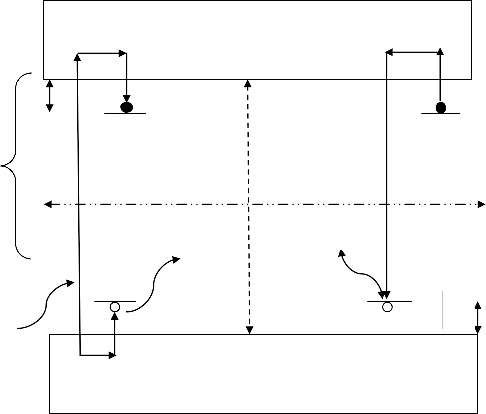
Moreover, figure1.B, shows the effect of heating, when the free electron absorbs enough energy, it to be released back into the conduction band, from where recombination is possible and accompanied by the release of a light emission[3].
Where the a is generation of holes and electrons, the b is electron trapping, the C is hole trapping, the d is electron release by heating, the R is recombination center with light emission, the is activation energy or trap depth, the g is hole trap depth, the Ef is Fermi level and thus
empty in the equilibrium state, and the Eg is forbidden energy.
IJSER © 2012 http://www.ijser.org
International Journal of Scientific & Engineering Research, Volume 3, Issue 10, October-2012 4
ISSN 2229-5518
Arrhenius's equation was described the probability per unit of release of an electron from a trap and considered that the electrons in the trap have a Maxwellian distribution of thermal energies.![]()
{ } (1)
Where:
The is Boltzmann’s constant=8.617*10-5 eV/k, the is absolute temperature ( ), the is the trap depth or activation energy (eV), the is frequency factor (not temperature dependent), depending on the frequency of the number of hits of an electron in the trap.
Randall and Wilkins, in 1945 assumed a mathematical expression for a peak in a glow curve. Their expressions were based on the energy band model and the well-known first -order kinetics [4].
If the temperature and number of trapped electrons in the trap are kept constant. Thus, the decreases with time by the following expression:![]()
…(2)
Integrating Eq.(2) one obtains![]()
n = no { ( ) } …(3)
Where no is the number of trapped electrons at the initial time =0
IJSER © 2012 http://www.ijser.org
International Journal of Scientific & Engineering Research, Volume 3, Issue 10, October-2012 5
ISSN 2229-5518
Assuming now the following assumptions [5]:
• No electrons are released from the trap, when irradiation of the thermoluminescent material was a low enough temperature.
• In recombination centers, the luminescence efficiency is no dependent on temperature.
• The recombination centers and concentrations of traps are no dependent on temperature.
• In the conduction band, the life time of the electrons is short
• Negligible retrapping during the heating stage
According to mentioned assumptions, at a constant temperature, the intensity of luminescence emission becomes directly proportional to the rate of release of electrons from the trap, :![]()
= ...(4)
Where is a constant proportionality. Eq.(4) is the equation of the decay phosphorescence at a constant temperature. For a linear increase in temperature at rate, , one obtains![]()
![]()
![]()
![]()
I(T) = = no s exp{ } exp{ ∫ { } }…….(5)
In 1948 Garlick and Gibson [6], they assumed in research of phosphorescence that two probabilities for a free charge carrier either recombination or being trapped within a
IJSER © 2012 http://www.ijser.org
International Journal of Scientific & Engineering Research, Volume 3, Issue 10, October-2012 6
ISSN 2229-5518
recombination center. The term second order kinetic is utilized to explain a behavior in which retrapping is present.
They suggested that when electron escaping from the trap has equal probability of either being recombining or retrapped of with a hole in a recombination centre.
![]()
![]()
I(T) = { }…..(6)
Where is called pre-exponential factor and constant; it is having dimensions of cm3sec-1.
Under temperature’s rise, the luminescence intensity of an irradiated phosphor is obtained from Eq.(6), introducing a linear heating rate , then the equation is obtained
![]()
![]()
![]()
I (T) = { }
![]()
![]()
![]()
∫ ( )
...(7)
The first or second order kinetics do not explain the actual glow peak, so, in (1964), May and
Partridge [7] suggested a general-order expression to cover several cases.![]()
![]()
![]()
![]()
I (T) = no exp{ } [ ∫ { } ] -b/b-1 ……..(8)
Where is s˝: sˊn0(b-1) with unit s-1
IJSER © 2012 http://www.ijser.org
International Journal of Scientific & Engineering Research, Volume 3, Issue 10, October-2012 7
ISSN 2229-5518
Eq.(8), it is help to deal with intermediate cases, and smoothly to first and second-orders when a nd , respectively.
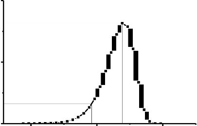
Garlick and Gibson (1948) were first suggested initial rise method of analysis, and assumed that the amount of trapped electrons in the low temperatures tail of glow peak can be approximately constant (i.e., for very little detrapping to have take place). In equation (5), the first exponential increases and value of the second term remain close to unity with the increase in temperature. Only upon an increase in temperature beyond a critical value , does this assumption become invalid (see. Figure2.). Furthermore, the temperature Tc must not correspond to an intensity which is more than approximately 10-15% of the maximum intensity [2].![]()
According to this suggestion of constant , the emission can be display by exp(- ) …………..(9)
For the applicability the initial rise method technique, the straight line is obtained when a plotting against The is calculated from the slope of the line without any knowledge of the S [8].
IJSER © 2012 http://www.ijser.org
International Journal of Scientific & Engineering Research, Volume 3, Issue 10, October-2012 8
ISSN 2229-5518
T
M
I
C
T
M
Temperature
Figure 2. The initial rise part of a thermoluminescence glow curve .
In 1980 [9], McKeever was suggested an alternative method, ie by “heating a previously irradiated sample at a linear rate up to a temperature corresponding to a point on the low temperature tail of the first peak. The sample is then cooled rapidly to room temperature and reheated, at the same linear rate, to record all of the remaining glow-curve. The position of the first maximum is noted. The process is repeated (on a freshly irradiated sample) using a new value of . ( is increased in small steps by 2 to 3 degrees) by noting the value of a plot of Tm versus is made”. The method is applied to first-order peaks and second-order glow-curves. Moreover, the technique proved to be particularly useful in pinpointing the individual peaks which were not obvious in the original glow-curve. Thus, only estimates of the true peak positions are given -the values are usually higher than the actual positions because
of peak overlap.
IJSER © 2012 http://www.ijser.org
International Journal of Scientific & Engineering Research, Volume 3, Issue 10, October-2012 9
ISSN 2229-5518
The estimation of trap depth based on the temperatures of the maxima are of two basic types. First, the direct relationship between and . Second, the change in caused by changing the rate which the sample is heated (heating rate method).
Randall and Wilkins in [1], they suggested that at the probability of charge release from a trap is unity![]()
( ) …(10)
Or
They were found expression for E, using a value =2.9* 109 S-1
… (11)
Urbach in 1930, displayed the similar relation using S=2.9* 109 S-1![]()
…(12)
The equations mention above can be used only as a first approximation of the E-values.
IJSER © 2012 http://www.ijser.org
International Journal of Scientific & Engineering Research, Volume 3, Issue 10, October-2012 10
ISSN 2229-5518
The maximum temperature of the peak's change related to heating rate changes: at quicker heating rates correspond a shift temperature about higher rate of .
Bohum, Porfianovitch and Booth [10, 11, 12], suggested that the method to calculate based on two different heating rates for a first-order peak.![]()
![]()
![]()
E = K [ ( ) ] …(13)
In 1958 [13], Hoogenstraaten was suggested the use of several heating rates to first-order equation for obtain the following linear relation.![]()
![]()
![]()
ln( +ln( ) ……(14)
Chen and Winer [14] displayed a method which uses almost to integral general-order expression of obtaining for equation![]()
![]()
ln[ ] ……………..(15) Where c is constant.
IJSER © 2012 http://www.ijser.org
International Journal of Scientific & Engineering Research, Volume 3, Issue 10, October-2012 11
ISSN 2229-5518
This method is based on the shape of the peak use two or three points from the glow-curve. Generally, these are the maximum of the peak , low-temperature and high temperature
(as shown in figure.3). However, the methods are depend on the order of kinetic. Where the:
is the half-width at the low temperature side of the peak, is the half-width toward the fall-off side of the glow peak, is the total half-width and the is the so-called geometrical shape or symmetry factor.
In (1953), Grossweiner was suggested first method to determine the trap depth kinetics [15].![]()
E= 1.51 K ……. (16) This expression explained on the first-order kinetics
For the first- and second-order kinetics, Lushchik was proposed method to calculate the [16].
For the first –order kinetics,![]()
E= …..(17) To second-order kinetics,![]()
E= ….(18)
Chen was modified equation mention above, by multiplying the 0.978, and 0.853 to equation
(17,18) respectively [17].
IJSER © 2012 http://www.ijser.org
International Journal of Scientific & Engineering Research, Volume 3, Issue 10, October-2012 12
ISSN 2229-5518
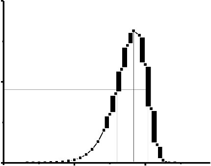
IM
T1 TM T2
Halperin and Braner produced a new formula by using the and on the glow curve.![]()
E= for first order …..(19)
![]()
E= for second order …..(20) With
![]()
IJSER © 2012 http://www.ijser.org
International Journal of Scientific & Engineering Research, Volume 3, Issue 10, October-2012 13
ISSN 2229-5518
Chen overcome the difficulty of the expression developed by Halperin and Braner which requires iterative process to find . The new developed expression is given as![]()
E = for first order ….(21)
![]()
E = for second order …(22)
Chen developed expressions to evaluate ; this method does not use any iterative processes and no need any knows to the kinetic order [18].![]()
E = ( ) - 2K ) …(23)
Where is , , or . The parameters of and are obtained as below:
=1.510 +3.0( = 1.58+4.2( - 0.42)
= 0.976+7.3( = 0
= 2.52+10.2( = 1,
Where =0.42 and =0.52 for the first order and the second order peaks respectively.
IJSER © 2012 http://www.ijser.org
International Journal of Scientific & Engineering Research, Volume 3, Issue 10, October-2012 14
ISSN 2229-5518
The method is to establish the approximate positions of the most prominent peaks in the glow- curve and to estimate initial values of , and by using one of the analytical methods. The method requires a numerical procedure for solving integral for first-order glow peaks is![]()
F (T, E) = ∫ { } …(24)
The integral can be solve by successive integration by parts to be equal to [19]![]()
![]()
F (T, E) = T { } ∑ ( ) …(25)
By application the first two terms in this approximation, the equation become![]()
![]()
![]()
F(T,E) = { } …(26)
The expression can be derived for the intensity glow curves, by using the approximation to the integral and the temperature for the maximum intensity to first -order equation.![]()
![]()
![]()
![]()
![]()
![]()
![]()
[ ( ) ]…(27)
During the second- and general-order TL glow curves, can obtain the general approximation by using series approximation![]()
![]()
![]()
![]()
![]()
![]()
![]()
( ) [ ( ) ( ) ] …(28)
IJSER © 2012 http://www.ijser.org
International Journal of Scientific & Engineering Research, Volume 3, Issue 10, October-2012 15
ISSN 2229-5518
![]()
![]()
![]()
![]()
![]()
![]()
![]()
![]()
[ ( ) ( ( ))] …(29)
Equation (29), to calculate the activation energy for general-order kinetics by using a curve fitting procedure.
The principle of thermoluminescence (TL) have been explained using simple model. The model illustrates of recombination and trap is necessary for the TL production. Furthermore, the model reveals how energy is stored. In addition, the glow peaks analysis has been for several methods, Initial Rise, Peak Position, Peak shape and Curve Fitting. Thus, the peak shape gives simple method does not use any iterative processes and no need any knows to the kinetic order.
[1] McKeever, 1985 S.W.S.McKeever,” Thermoluminescence of solids”. Cambridge University,
Cambridge(1985).
[2] Bos, A.J.J. (2007).”Theory of thermoluminescence”. Radiation measurements, 41, s45-s56.
[3] Furetta, C. (2003).”Handbook of thermoluminescence”. World scientific, Singapore. [4] Randall. J.F.G and Wilkins. M.H.F, proc. Roy. Soc. A184 (1945)366.
[5] Furetta, C.(2005).”Model and methods thermoluminescence”. Conference, 7-9 Septiembre de Zacatecas, Zac. México.
[6] G.F.J. Garlick and A.F.Gibson,Proc.Phys.Soc.60(1948)574.
IJSER © 2012 http://www.ijser.org
International Journal of Scientific & Engineering Research, Volume 3, Issue 10, October-2012 16
ISSN 2229-5518
[7] May. C.E. and J.A. Partridge, J. Chem.Soc.40(1964)1880. [8] Ilich. B.M.(1979). Sov. Phys. Solid State, 21, 1880.
[9] McKeever. S.W.S.(1980). Phys. Stat. Solidi (a), 62, 331 [10] Bohum. A.(1954). Czech. J. Phys. 4, 91.
[11] Porfianovitch. I. A. (1954). Exp.J. Theor. Phys. USSR 26, 696. [12] Booth. A.H.(1954). Canad. J. Chem. 32, 214.
[13] Hoogenstraaten. W. (1958). Philips Res. Rep, 515.
[14] Chen. R and Winner. S. A. A.(1970). J. Appl. Phys. 4,1 5227. [15] Grossweiner. L.I. (1953). J. Appl. Phys. 24, 1306.
[16] Lushihik L.I. (1956). Soviet Phys. JEPT 3, 390. [17] Chen. R. (1969). J. Appl. Phys. 40, 570.
[18] Chen. R. (1969). J. Electrochem. Soc. 116, 1254.
[19] Kitis. G, Gomez-Ros. J.M, and Tuyn. J.W.N. (1998). J. Phys. D 31, 2636
IJSER © 2012 http://www.ijser.org