International Journal of Scientific & Engineering Research, Volume 4, Issue 5, May 2013
ISSN 2229‐5518
Sayaji Rastum Waykar
(Research Scholar, JJT, University, Rajasthan) Assistant Professor, Department of Mathematics Yashwantrao Chavan Mahavidyalaya, Halkarni
Tal: Chandgad, Dist: Kolhapur, Maharashtra (India).
Email:
The paper will consist of three parts. In part‐I, we shall present some background considerations which are necessary as a basis for what follows. We shall try to clarify some basic concepts and notions and we shall collect the most important arguments and related goals in favor of problem solving modeling and applications to other subjects in mathematics instructions. In the main part‐II we shall review the present state, recent trends and prospective lines of development, both in empirical or theoretical research and in the practice of mathematics education, concerning applied problem solving, modeling, applications and relations to other subjects. In particular, we shall identify and discuss four major trends; a widened spectrum of arguments, an increased globality, an increased unification and an extended use of computer. In the final Part‐III, we shall comment upon some important issues and problems related to our topic.
Also, In this paper; I will discuss on Mathematical modeling. It means the process of translation between the real world and Mathematics in the both directions is one of the topics in Mathematics education that has been discussed and propagated most intensely during last few decades. The number of papers and research reports addressing the theory and/or practice of mathematical modeling with some form of connection to education is growing astronomically.
So, I say mathematical modeling is a way of life.
Applied Mathematical modeling welcomes contributions on research related to the mathematical modeling of engineering and environmental processes, manufacturing and industrial systems. A significant emerging area of research activity involves multi‐physics processes and contributions in this area are particularly encouraged. Applied mathematical
modeling is aimed at reflecting the advances of what is a very fast moving area of endeavor. All
IJSER © 2I013 http://www.ijser.org
International Journal of Scientific & Engineering Research, Volume 4, Issue 5, May 2013
ISSN 2229‐5518
engineering organizations make extensive use of computational models in the design analysis, optimization and control of processes or systems. The objective of the paper is to serve the needs of the mathematical modeling community by acting as the focus for the communication of research results, reviews of progress and discussions of issues of emerging interest to those in this rapidly expanding field.
Mathematical Modelling or what is mathematical modelling? :
Begin with observations.
Based on observation, construct a mental image or model.
Use the model to make predictions and test those predictions by doing new experiments.
If necessary, revise the model.
Repeat the last two steps above, as necessary, to obtain better models.
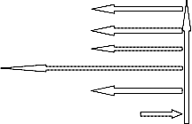
A diagrammatic Interpretation of mathematical modeling process is shown figure‐1.![]()
The arrows on the left display the ultimate pathway from problem setting to solution , while those on the right indicate that iterative back tracking may occur repeatedly between any phases of the mathematical modeling cycle –whenever such a need is identified. This is a compact version of the mathematical modeling framework.
To support the research focus the basic mathematical modeling framework was elaborated into what for purposes of distinction is called a mathematical modeling diagram. Also it has seven stages of modeling cycle. It serves to define and via its structure and the attached box identify‐ key foci for research with respect to individuals learning mathematical modeling and pressure points for those teaching within the field . For example, the kinds of mental activity that individuals engage in as modellers attempting to make the transition from one modeling stage
to the next and which provide key foci for research are given by the following:
IJSER © 2I013 http://www.ijser.org
International Journal of Scientific & Engineering Research, Volume 4, Issue 5, May 2013
ISSN 2229‐5518

1. Understanding , structuring, simplifying, interpreting context
2. Assuming, formulating, mathematising
3. Working mathematically
4. Interpreting mathematical output
5. Comparing, critiquing, validating
6. Communicating, justifying (if model is deemed satisfactory)
7. Revisiting the modeling process (if model is deemed unsatisfactory)
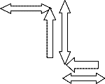
Another of Mathematical modeling cycle is shown in fig‐2 as follows:![]()
![]()
![]()
![]()
Situation statement ![]()
![]()
solution Accept solution of solution solution
The light double‐headed arrows emphasis that thinking within the modeling process is far from linear and indicate the presence of reflective metacognitive activity as articulated by many researchers .Such reflective activity can look both forwards and backwards with respect to stages in the modeling process.
cognitive analyses of modelling tasks is a model of the “modelling cycle” for solving these tasks.
Here is the seven‐step model that I use in both my projects.
A modelling task requires translations between reality and Mathematics what, in short, can be called mathematical modelling. By reality, I mean according to Pollak (1979), the “rest of the
IJSER © 2I013 http://www.ijser.org
International Journal of Scientific & Engineering Research, Volume 4, Issue 5, May 2013
ISSN 2229‐5518
world” outside mathematics including nature, society, everyday life and other scientific disciplines. So by seven steps model is as follows: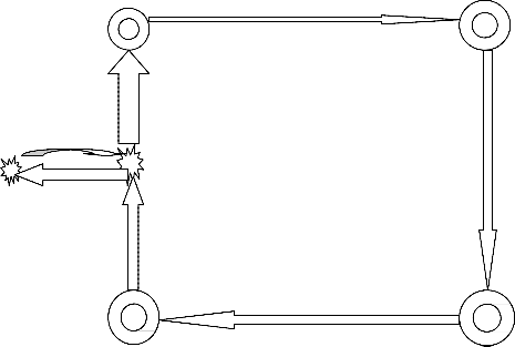
Real model & problem mathematical model & problem
Real situation 1 situation model
& problem 7
Real results Mathematical results
model iii) using mathematics iv) explaining result.
![]()

![]()
1. Understanding task 2. Establishing model
a) Read the text precisely and a) Look for the data you need. If
Imagine the situation clearly. necessary: make assumptions![]()
![]()
b) Make a sketch b) Look for mathematical relations![]()
![]()
4. Explaining result 3. Using mathematics
a) Round off and link the result to a) Use appropriate procedures task. If necessary, go back to 1 b) Write down your mathematical
b) Write down your final answer result.
IJSER © 2I013 http://www.ijser.org
International Journal of Scientific & Engineering Research, Volume 4, Issue 5, May 2013
ISSN 2229‐5518
I have observed that from figure 1 to 4 shows that the various types for writing the real situation in the form of a modeling cycle or modeling process. This is known as mathematical modelling.
I have all seen presentations made with a projector that has been tilted by putting books under the front so that the projected image is high enough on the screen. The projected image is distorted wider at the top than at the bottom. The reason is that the slide and the screen are
not parallel. This is our first model for the behavior of light and shadows. I can’t actually see what is happening between the light source and the slide and then between the slide and the wall but I have formed a mental picture or model of what is happening and that model enables me to make predictions that can then be verified or contradicted by experimental evidence.
There are more than 176 co‐operative sugar factories and 52 sugar mills in the state Maharashtra. With more than one –third of the co‐operative sugar factories in the state being sick, the Maharashtra government had appointed an expert committee to go into the reasons for the sickness and to suggest remedial measures. In view of the importance of the co‐ operative sugar industry for Maharashtra’s economy as well as the relevance of the expert committees recommendations for co‐operative sugar factories in a number of other states,
these recommendations deserve to be discussed widely.
As on June 30, 1961, co‐operative institutions of various kinds –agricultural and non agricultural primary co‐operative societies, marketing societies, processing co‐operative societies and
others in Maharashtra totaled 31,565. Today, this number progressively went up to more than
146641 to 227000. The co‐operative sector is worrisome since it plays an important role in the economy of a number of states.
Maharashtra is in the forefront of these states. However, all is not well with the co‐operative movement in Maharashtra. Of the co‐operatives as above, 43744 co‐operatives incurred loss as compared with 47292 co‐operatives which made profit and 2923 co‐operatives neither made profit nor incurred loss while information in respect of 45536 co‐operatives was not available.
IJSER © 2I013 http://www.ijser.org
International Journal of Scientific & Engineering Research, Volume 4, Issue 5, May 2013
ISSN 2229‐5518
Therefore, I observed that the maximum co‐operative Institutes or sugar factories being sick because a lot of corruption in it.
Here, I use seven steps mathematical modelling cycle. The Shetakari Co‐operative Sugar Factory, Dadanagar was established on 1978‐79 and first production on the year 1980‐81 was 5 lakh quintal sugar and its cost Rs.50 crore (Rs.10 each kg.). Therefore, total income was Rs.50 crore per 3 years period because this factory was multi‐state.
Suppose, initially corruption was zero when t=0 on the time of first production that was on October/November 1980. After three years period corruption was one percentage of total income of first production that was 0.50 crore on the time oct/nov‐1983.
Now, we know that the mathematical corruption growth formula,![]()
C = ![]()
![]() ‐‐‐‐‐‐‐‐‐‐‐‐‐‐‐‐‐‐‐‐‐‐‐‐‐‐‐‐‐ (i)
‐‐‐‐‐‐‐‐‐‐‐‐‐‐‐‐‐‐‐‐‐‐‐‐‐‐‐‐‐ (i)
Therefore, corruption C=0.50 crore, when t=3 years period on the time oct/nov‐1983.![]()
From (i), 0.50= ![]()
![]() ‐‐‐‐‐‐‐‐‐‐‐‐‐‐‐‐‐‐‐‐‐‐‐‐‐‐‐‐‐‐ (ii) But we take E‐virus Ҝ =0, we have
‐‐‐‐‐‐‐‐‐‐‐‐‐‐‐‐‐‐‐‐‐‐‐‐‐‐‐‐‐‐ (ii) But we take E‐virus Ҝ =0, we have
![]()
From (ii), 0.50= ![]()
![]()
![]() = 0.50 crore
= 0.50 crore
Therefore, putting this value in equation (i), we have![]()
C=0.50 ![]() ‐‐‐‐‐‐‐‐‐‐‐‐‐‐‐‐‐‐‐‐‐‐‐‐‐‐‐‐‐‐‐‐‐‐ (iii)
‐‐‐‐‐‐‐‐‐‐‐‐‐‐‐‐‐‐‐‐‐‐‐‐‐‐‐‐‐‐‐‐‐‐ (iii)
After three years period, that was time oct/nov‐1986. Corruption was double of previous period, that was C=1 crore, when t=3 years.
Putting in equation (iii), we have![]()
1=0.50 ![]()
![]()
![]()
=![]() =2
=2![]()
![]()
=![]()
IJSER © 2I013 http://www.ijser.org
International Journal of Scientific & Engineering Research, Volume 4, Issue 5, May 2013
ISSN 2229‐5518
Putting in equation (iii), we have![]()
C=0.50 ![]() ‐‐‐‐‐‐‐‐‐‐‐‐‐‐‐‐‐‐‐‐‐‐‐‐‐‐‐‐ (iv) Note that in the both the cases of the above, we take E‐virus Ҝ =0.
‐‐‐‐‐‐‐‐‐‐‐‐‐‐‐‐‐‐‐‐‐‐‐‐‐‐‐‐ (iv) Note that in the both the cases of the above, we take E‐virus Ҝ =0.
Now when next three years period that is t=9 years from base, then what was C=? at oct/nov‐
1989.![]()
From (iv), C=0.50 ![]()
![]()
C=0.50 ![]()
![]()
![]()
C=0.50 8![]()
At the time oct/nov‐1992, t=12 years, what was C =?![]()
From (iv), C=0.50 ![]()
![]()
C=0.50 ![]()
![]()
![]()
C=0.50 16![]()
At the oct/nov‐1995, t=15 years, what was C=?![]()
From (iv), C=0.50 ![]()
![]()
C=0.50 ![]()
![]()
![]()
C=0.50 32![]()
At the oct/nov‐1998, t=18 years, what was C=?![]()
From (iv), C=0.50 ![]()
IJSER © 2I013 http://www.ijser.org
International Journal of Scientific & Engineering Research, Volume 4, Issue 5, May 2013
ISSN 2229‐5518
![]()
![]()
C=0.50![]()
![]()
C=0.50 64![]()
At the oct/nov‐2001, t=21 years, what was C=?![]()
From (iv), C=0.50 ![]()
![]()
C=0.50 ![]()
![]()
![]()
C=0.50 128![]()
At the oct/nov‐2004, t=24 years, what was C=?![]()
From (iv), C=0.50 ![]()
![]()
C=0.50 ![]()
![]()
![]()
C=0.50 256![]()
At the oct/nov‐2009, t=29 years, what was C=?![]()
From (iv), C=0.50 ![]()
![]()
C=0.50 ![]()
![]()
![]()
C=0.50 812.7681![]()
Therefore, I have observed that today, the corruption in the Shetakari co‐operative sugar factory, Dadanagar is approximately Rs. 406.3840 crore.
From the above, we have seen that first we understand the real world problem situation‐
Corruption in co‐operatives then we get corruption problems statement after that we formed
IJSER © 2I013 http://www.ijser.org
International Journal of Scientific & Engineering Research, Volume 4, Issue 5, May 2013
ISSN 2229‐5518
mathematical corruption model and then we get a mathematical results or mathematical solution. Then this mathematical solution compare or validity with reality of the real world. Again, revise the model for a accurate solution. This is a seven stage mathematical modeling cycle.
The above data can be written in the tabular form as of the following:
Time t (years) | ‐ve corruption | Actual value of C | +ve corruption |
0 | 0 | 0 | 0 |
3 | 0.50 | 0.50 | 0 |
6 | 1.00 | 2.00 | 1.00 |
9 | 1.50 | 4.00 | 2.50 |
12 | 2.00 | 8.00 | 6.00 |
15 | 2.50 | 16 | 13.50 |
18 | 3.00 | 32 | 29.00 |
21 | 3.50 | 64.00 | 60.50 |
24 | 4.00 | 128.00 | 124.00 |
29 | 5.00 | 406.3840 | 401.3840 |
The graph of Mathematical corruption of the above data is as follows:
IJSER © 2I013 http://www.ijser.org
International Journal of Scientific & Engineering Research, Volume 4, Issue 5, May 2013
ISSN 2229‐5518
I have observed that the negative corruption decreases and positive corruption increases. Therefore, the Shetakari co‐operative sugar factory, Dadanagar will become very sick or very weak. That is why we say all is not well with the co‐operative movement in M‐ashtra.
We know that the total population of M‐ashtra was 3.0 crore (approximately) at 15 August,
1947 (freedom date).
Suppose, I assume that there was no corruption in the M‐ashtra at that time. Therefore, corruption C=0, when t=0.
After 10 years, 15 August, 1957, corruption was one percentage of old population, that is 0.03
crore.
We know that the mathematical corruption growth formula,![]()
C = ![]()
![]() , Ҝ > 0. ‐‐‐‐‐‐‐‐‐‐‐‐‐‐‐‐‐‐‐‐‐‐‐‐‐‐‐ (i)
, Ҝ > 0. ‐‐‐‐‐‐‐‐‐‐‐‐‐‐‐‐‐‐‐‐‐‐‐‐‐‐‐ (i)
![]()
0.03 = ![]()
But we take, Ҝ=0 we have![]()
0.03 = ![]()
![]()
![]()
![]()
0.03 = ![]() , where
, where ![]() =1
=1 ![]() =0.03 crore.
=0.03 crore.
Putting in (i), we get![]()
Therefore from equation (ii), 0.06=0.03 ![]()
IJSER © 2I013 http://www.ijser.org
International Journal of Scientific & Engineering Research, Volume 4, Issue 5, May 2013
ISSN 2229‐5518
![]()
![]()
![]() =
=
![]()
![]() =
=
![]()
From (ii), we have![]()
![]()
This is a Mathematical basement corruption formula. When t= 30 years from base at 15 August, 1977. Therefore from equation (iii), we have![]()
![]()
![]()
![]()
![]()
When t=40 years from base at 15 August, 1987. Therefore from equation (iii), we have![]()
![]()
![]()
![]()
![]()
When t=50 years from base at 15 August, 1997. Therefore from equation (iii), we have![]()
![]()
IJSER © 2I013 http://www.ijser.org
International Journal of Scientific & Engineering Research, Volume 4, Issue 5, May 2013
ISSN 2229‐5518
![]()
![]()
![]()
When t=60 years from base at 15 August, 2007. Therefore from equation (iii), we have![]()
![]()
![]()
![]()
![]()
When t=65 years from base at 15 August, 2012. Therefore from equation (iii), we have![]()
![]()
![]()
![]()
![]()
![]()
When t=70 years from base at 15 August, 2017. Therefore from equation (iii), we have![]()
![]()
![]()
![]()
![]()
When t=80 years from base at 15 August, 2027.
IJSER © 2I013 http://www.ijser.org
International Journal of Scientific & Engineering Research, Volume 4, Issue 5, May 2013
ISSN 2229‐5518
Therefore from equation (iii), we have![]()
![]()
![]()
![]()
![]()
When t=90 years from base at 15 August, 2037. Therefore from equation (iii), we have![]()
![]()
![]()
![]()
![]()
When t=100 years from base at 15 August, 2047. Therefore from equation (iii), we have![]()
![]()
![]()
![]()
![]()
Time t (years) | 0‐10 | 10‐20 | 20‐30 | 30‐40 | 40‐50 | 50‐60 | 60‐70 | 70‐80 | 80‐90 |
Corruption C (crore) | 0.03 | 0.06 | 0.24 | 0.48 | 0.96 | 1.92 | 3.84 | 7.68 | 15.36 |
IJSER © 2I013 http://www.ijser.org
International Journal of Scientific & Engineering Research, Volume 4, Issue 5, May 2013
ISSN 2229‐5518
We assume that there was no corruption on 15 August, 1947 (Freedom date). Therefore C=0 and Development was one percentage of old population.
That is when C=0, D = D(0) =![]() =0.03 crore
=0.03 crore
After 10 years from freedom that is 15 August, 1957, C = 0.03 crore and
The Development would be double of old that is D(c) =0.06 crore. We know that MGD‐Model,
D(c) = D(0) ![]() ‐‐‐‐‐‐‐‐‐‐‐‐‐‐‐‐‐‐‐‐‐‐‐ (i)
‐‐‐‐‐‐‐‐‐‐‐‐‐‐‐‐‐‐‐‐‐‐‐ (i)![]()
0.06 =D(0) ![]()
But we take Ҝ =0, where Ҝ be the E‐virus lead to increase the corruption![]()
0.06 = D(0) ![]()
![]()
![]()
0.06 = D(0) 1![]()
D(0) = 0.06
Putting this value in equation (i), we have![]()
D(c) = 0.06 ![]() ‐‐‐‐‐‐‐‐‐‐‐‐‐‐‐‐‐‐‐‐ (ii)
‐‐‐‐‐‐‐‐‐‐‐‐‐‐‐‐‐‐‐‐ (ii)
After 20 years from freedom, C = 0.06 crore and Development would be double of old that is D = 0.12 crore, putting in (ii), we have![]()
0.12 = 0.06 ![]()
![]()
![]()
![]()
= ![]()
![]() = 2
= 2
![]()
![]()
![]()
= [ ![]()
Ҝ=
IJSER © 2I013 http://www.ijser.org
International Journal of Scientific & Engineering Research, Volume 4, Issue 5, May 2013
ISSN 2229‐5518
Putting in (ii), we have![]()
![]()
This is a Mathematical basement formula for development of related corruption.
After 30 years (15 August 1977) from freedom when corruption C= 0.24 crore, D(C) =?![]()
From (iii), D(c) = 0.06 [ ![]()
![]()
=0.06 [ ![]()
![]()
![]()
After 40 years (15 August 1987) from freedom when corruption C= 0.48 crore, D(c) =?![]()
From (iii), D(c) = 0.06 [ ![]()
![]()
![]()
![]()
After 50 years (15 August 1997) from freedom when corruption C=0.96 crore, D(c) =?![]()
From (iii), D(c) = 0.06 [ ![]()
![]()
![]()
= 0.06 65536![]()
![]()
After 60 years (15 August 2007) from freedom when corruption C=1.92 crore, D(C) =? From (iii), D(c) = 0.06 [ ![]()
IJSER © 2I013 http://www.ijser.org
International Journal of Scientific & Engineering Research, Volume 4, Issue 5, May 2013
ISSN 2229‐5518
![]()
![]()
= 0.06 65536 65536![]()
![]()
From (iii), D(c) = 0.06 [ ![]()
![]()
![]()
=0.06 4.1784e+013![]()
After 70 years (15 August 2017) from freedom when corruption C=3.84 crore, D(c) =?![]()
From (iii), D(c) = 0.06 [ ![]()
![]()
![]()
![]()
=0.06 [![]() [
[ ![]()
![]()
Here, I have to use Applied Mathematical method. In this method I use initial values and Mathematical Growth formula for finding Mathematical Growth of Development Model. A slightly more realistic and largely used mathematical growth model is the logistic function and its extensions.
In the above data, I have observed that the development of such persons which have corrupted. This result on present situations because a lot of corruption ghotales are opens.
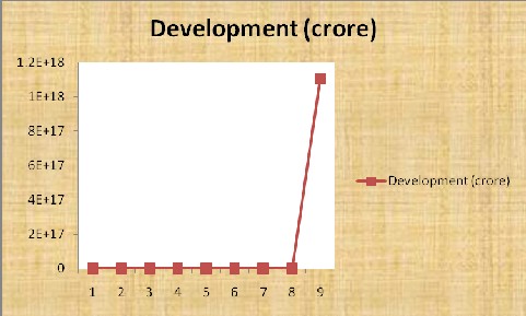
I have found the values of Development (general) related to the Corruption are in the tabular form:
Time (years) | Corruption (crore) | Development (crore) |
15 August,1947 | 0 | 0.03 |
15 August,1957 | 0.03 | 0.06 |
IJSER © 2I013 http://www.ijser.org
International Journal of Scientific & Engineering Research, Volume 4, Issue 5, May 2013
ISSN 2229‐5518
15 August,1967 | 0.06 | 0.12 |
15 August,1977 | 0.24 | 0.96 |
15 August,1987 | 0.48 | 15.36 |
15 August,1997 | 0.96 | 3932.16 |
15 August,2007 | 1.92 | 257698037.76 |
15 August,2012 | 2.71488 | 2.5070e+012 |
15 August,2017 | 3.84 | 1.1068e+018 |
The above table shows the Corruption and related Development in crores. Also I have observed that the Corruption increases and the Development decreases in the M‐ashtra, India. The result of Corruption and Development shows the reality of the present situation in the M‐ashtra,
India.
of the above result‐
5.1 is as follows:
I have observed and it concluded that the mathematical modeling process is used in the above two results. That means first understand the real world problems situation. That is ‘corruption’ situation then frame appropriate mathematical questions: i) what is corruption? ii) How does it remove from society? iii) Advantages and disadvantages of corruption? Then formulate a
model, using simplifying assumptions and analyze the model. So I have found mathematical
IJSER © 2I013 http://www.ijser.org
International Journal of Scientific & Engineering Research, Volume 4, Issue 5, May 2013
ISSN 2229‐5518
corruption model. Then we get mathematical result when we compare this mathematical result with real life result of the society. Mathematical modeling affords reflecting on mathematical concepts and their roles for solving real‐world problems as well as creating rich learning opportunities. As Pollack (1979, P.240) states, modeling, ‘requires an understanding of the situation outside mathematics and of the process of mathematisation as well as of the mathematics itself ’. Conversely, the role of mathematics can be recognized particularly clearly when reflecting on modeling processes. The contribution of mathematical ideas and concepts can be made transparent for learners through their use in modeling real‐world problems. So we solve any problems of any fields by using Mathematical modelling. Therefore we say Mathematical modelling is a way of life.
[1]. Borromeo Ferri, R. (2007). Modelling problems from a cognitive perspective. In: Haines, C. et al. (Eds), Mathematical Modelling : Education, Engineering and Economics. Chichester: Horwood, 260270.
[2]. Blum, W. / Niss, M. (1991). Applied mathematical problem solving, modeling, applications, and links to other subjects‐ state, trends and issues in mathematics instruction.
In: Educational studies in Mathematics, 22(1), 37‐68.
[3]. Blum, W. et. Al.(2002). ICMI study 14: Applications and Modelling in Mathematics
Education‐Discussion document. Educational Studies in Mathematics, 51(1/2), 149‐171. [4]. Blum, W. / Galbraith, P. / Henn, H. W. / Niss, M. (Eds. 2007). Modelling and Applications in
Mathematics Education. New York: Spring.
[5]. De Lange, J. (1996). Real problems with real world mathematics. In L. Alsina & al. (Eds.), Proceeding of the 8th Int. Congress on Math.1 Education (PP. 83‐110). Sevilla: Thales.
[6]. DaPonte, J. P. (1993). Necessary research in Mathematical modeling and applications. In: Breiteig, T. et. al.(Eds.),Teaching and Learning Mathematics in context. Chichester: Horwood, 219‐227.
[7]. Schoenfeld A. H. (1994). Mathematical Thinking and Problem Solving. Hillsdale: Erlbaum. [8]. Shulman, L. (1986). Those who understand: Knowledge growth in teaching. Educational
Researcher, 15(2), 4‐14.
[9]. Verschaffel,L. / Greer, B. / DeCorte, E. (2000). Making sense of world Problems. Lisse: Swets
& Zeitlinger.
[10]. Zafar Ashan, Differential equations and their applications, prentice hall of India, New Delhi
(1999).
IJSER © 2I013 http://www.ijser.org