The research paper published by IJSER journal is about MEDICAL IMAGE COMPRESSION USING REGION GROWING SEGMENATION 1
ISSN 2229-5518
MEDICAL IMAGE COMPRESSION USING REGION GROWING SEGMENATION
R.Arun, M.E & D.Murugan Asst.
![]()
—————————— ——————————![]()
There are two types of image compression: lossless and lossy. With lossless compression, the original image is recovered exactly after decompression. Unfortunately, with images of natural scenes it is rarely possible to obtain error-free com- pression at a rate beyond 2:1. Much higher compression ratios can be obtained if some error, which is usually difficult to perceive, is allowed between the decompressed image and the original image. This is lossy compression. In many cases, it is not necessary or even desirable that there be error-free repro- duction of the original image. For example, if some noise is present, then the error due to that noise will usually be signifi- cantly reduced via some denoising method. In such a case, the small amount of error introduced by lossy compression may be acceptable. Another application where lossy compression is acceptable is in fast transmission of still images over the Inter- net.
Before the various image compression techniques are dis- cussed, consider the motivation behind using compression. A typical 12-bit medical X-ray may be 2048 pixels by 2560 pixels in dimension. This translates to a file size of 10,485,760 bytes. A typical 16-bit mammogram image may be 4500 pixels by
4500 pixels in dimension for a file size of 40,500,000 (40 mega- bytes)! This has consequences for disk storage and image transmission time. Even though disk storage has been increas- ing steadily, the volume of digital imagery produced by hos- pitals and their new film less radiology departments has been increasing even faster. Even if there were infinite storage, there is still the problem of transmitting the images.
An image is a collection of measurements in two-dimensional
(2-D) or three-dimensional (3-D) space. In medical images,
these measurements or image intensities can be radiation ab-
sorption in X-ray imaging, acoustic pressure in ultrasound, or
RF signal amplitude In MRI. If a single easurement is made at
each location in the image, then the image is called a scalar
image. With the growth of technology and the entrance into
the Digital Age, the world has found itself amid a vast amount
of information. Dealing with such enormous amount of infor-
mation can often present difficulties. Digital information must
be stored and retrieved in an efficient manner, in order for it to
be put to practical use. Data compression is a fascinating topic
when considered by it.
![]()
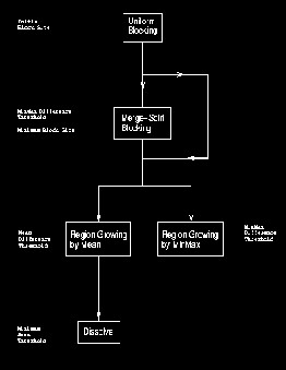
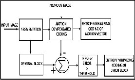
It refers to the process of partitioning a digital image into mul- tiple segments (sets of pixels, also known as super pixels). The goal of segmentation is to simplify and/or change the repre- sentation of an image into something that is more meaningful and easier to analyze. Image segmentation is typically used to locate objects and boundaries (lines, curves, etc.) in images. More precisely, image segmentation is the process of assigning a label to every pixel in an image such that pixels with the same label share certain visual characteristics
![]()
The first region growing method was the seeded region grow- ing method. This method takes a set of seeds as input along with the image. The seeds mark each of the objects to be seg-
IJSER © 2012
The research paper published by IJSER journal is about MEDICAL IMAGE COMPRESSION USING REGION GROWING SEGMENATION 2
ISSN 2229-5518
mented. The regions are iteratively grown by comparing all unallocated neighboring pixels to the regions. The difference between a pixel's intensity value and the region's mean, δ, is used as a measure of similarity. The pixel with the smallest difference measured this way is allocated to the respective region. This process continues until all pixels are allocated to a region.
Seeded region growing requires seeds as additional input. The segmentation results are dependent on the choice of seeds. Noise in the image can cause the seeds to be poorly placed. Unseeded region growing is a modified algorithm that doesn't require explicit seeds. It starts off with a single region A1 – the pixel chosen here does not significantly influence final seg- mentation. At each iteration it considers the neighboring pix- els in the same way as seeded region growing. It differs from seeded region growing in that if the minimum δ is less than a predefined threshold T then it is added to the respective re- gion Aj. If not, then the pixel is considered significantly differ- ent from all current regions Ai and a new region An + 1 is created with this pixel.
![]()
The EZW algorithm is based on four key concepts: 1) a dis- crete wavelet transform or hierarchical sub band decomposi- tion, 2) prediction of the absence of significant formation across scales by exploiting the self-similarity inherent in im- ages, 3) entropy-coded successive approximation quantiza- tion, and 4) universal lossless data compression which is achieved via adaptive Huffman encoding. The EZW encoder was originally designed to operate on images (2D-signals) but it can also be used on other dimensional signals. The EZW
encoder is based on progressive encoding to compress an im- age into a bit stream with increasing accuracy. This means that when more bits are added to the stream, the decoded image will contain more detail, a property similar to JPEG encoded images. Using an embedded coding algorithm, an encoder can terminate the encoding at any point thereby allowing a target rate or target accuracy to be met exactly. Also, given a bit stream, the decoder can cease decoding at any point in the bit stream and still produce exactly the same image that would have been encoded at the bit rate corresponding to the trun- cated bit stream. In addition to producing a fully embedded bit stream, EZW consistently produces compression results that are competitive with virtually all known compression algorithm on standard test images It is similar to the represen- tation of a number like π (pi). Every digit we add increases the accuracy of the number, but we can stop at any accuracy we like. Progressive encoding is also known as embedded encod- ing, which explains the E in EZW.
![]()
The embedded zerotree wavelet algorithm (EZW) is a simple, yet remarkable effective, image compression algorithm, hav- ing the property that the bits in the bit stream are generated in order of importance, yielding a fully embedded code. Using an embedded coding algorithm, an encoder can terminate the encoding at any point thereby allowing a target rate or target distortion metric to be met exactly. Also, given a bit stream, the decoder can cease decoding at any point in the bit stream and still produce exactly the same image that would have been encoded at the bit rate corresponding to the truncated stream. In addition to producing a fully embedded bit stream, EZW consistently produces compression results that are competitive with virtually all known compression algorithms.
The EZW output stream will have to start with some informa- tion to synchronize the decoder. The minimum information required by the decoder is the number of wavelet transform levels used and the initial threshold, if we assume that always the same wavelet transform will be used. Additionally we can send the image dimensions and the image mean. Sending the image mean is useful if we remove it from the image before coding. After imperfect reconstruction the decoder can then replace the imperfect mean by the original mean. This can in- crease the PSNR significantly.
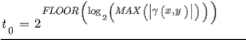
The first step in the EZW coding algorithm is to determine the initial threshold. If we adopt bitplane coding then our initial threshold t0 will be
IJSER © 2012
The research paper published by IJSER journal is about MEDICAL IMAGE COMPRESSION USING REGION GROWING SEGMENATION 3
ISSN 2229-5518
Here MAX(.) means the maximum coefficient value in the im- age and ![]() denotes the coefficient. With this threshold we enter the main coding loop (I will use a C-like language):
denotes the coefficient. With this threshold we enter the main coding loop (I will use a C-like language):
threshold = initial_threshold;
do
{
dominant_pass(image);
subordinate_pass(image);
threshold = threshold/2;
}
while (threshold>minimum_threshold);
We see that two passes are used to code the image. In the first pass, the dominant pass, the image is scanned and a symbol is outputted for every coefficient. If the coefficient is larger than the threshold a P (positive) is coded, if the coefficient is small- er than minus the threshold an N (negative) is coded. If the coefficient is the root of a zerotree then a T (zerotree) is coded and finally, if the coefficient is smaller than the threshold but it is not the root of a zerotree, then a Z (isolated zero) is coded. This happens when there is a coefficient larger than the thre- shold in the subtree. The effect of using the N and P codes is that when a coefficient is found to be larger than the threshold (in absolute value or magnitude) its two most significant bits are outputted (if we forget about sign extension).
Note that in order to determine if a coefficient is the root of a zerotree or an isolated zero, we will have to scan the whole quad-tree. Clearly this will take time. Also, to prevent output- ting codes for coefficients in already identified zerotrees we will have to keep track of them. This means memory for book keeping.
Finally, all the coefficients that are in absolute value larger than the current threshold are extracted and placed without their sign on the subordinate list and their positions in the im- age are filled with zeroes. This will prevent them from being coded again.
The second pass, the subordinate pass, is the refinement pass. In [Sha93] this gives rise to some juggling with uncertainty inter- vals, but it boils down to outputting the next most significant bit of all the coefficients on the subordinate list. In [Sha93] this list is ordered (in such a way that the decoder can do the same) so that the largest coefficients are again transmitted first. Based on [Alg95] we have not implemented this sorting here since the gain seems to be very small but the costs very high.
The main loop ends when the threshold reaches a minimum value. For integer coefficients this minimum value equals zero and the divide by two can be replaced by a shift right opera- tion. If we add another ending condition based on the number
of outputted bits by the arithmetic coder then we can meet any target bit rate exactly without doing too much work.
We can summarize the above with the following code frag- ments, starting with the dominant pass.
/*
* Dominant pass
*/
initialize_fifo();
while (fifo_not_empty)
{
get_coded_coefficient_from_fifo();
if coefficient was coded as P, N or Z then
{
code_next_scan_coefficient();
put_coded_coefficient_in_fifo();
if coefficient was coded as P or N then
{
add abs(coefficient) to subordinate list;
set coefficient position to zero;
}
}
}
Here we have used a FIFO to keep track of the identified zero- trees. If we want to enter this loop we will have to initialize the FIFO by ‚manually‛ adding the first quad-tree root coeffi- cients to the FIFO. Depending on which level we start in the left of figure 2 this means coding and putting at least three roots in the FIFO. The call of code_next_scan_coefficient() checks the next uncoded coefficient in the image, indicated by the scanning order and outputs a P, N, T or Z. After coding the coefficient it is put in the FIFO. This will automatically result in a Morton scan order. Thus, the FIFO contains only coefficients which have already been coded, i.e. a P, N, T or Z has already been outputted for these coefficients. Finally, if a coefficient was coded as a P or N we remove it from the image and place it on the subordinate list.
This loop will always end as long as we make sure that the coefficients at the last level, i.e. the highest subbands (HH1, HL1 and LH1 in figure 2) are coded as zerotrees.
After the dominant pass follows the subordinate pass:
/*
* Subordinate pass
*/
subordinate_threshold = current_threshold/2;
for all elements on subordinate list do
{![]()
if (coefficient>subordinate_threshold)
IJSER © 2012
The research paper published by IJSER journal is about MEDICAL IMAGE COMPRESSION USING REGION GROWING SEGMENATION 4
ISSN 2229-5518
{
output a one;
coefficient = coefficient-subordinate_threshold;
}
else output a zero;
}
If we use thresholds that are a power of two, then the subor- dinate pass reduces to a few logical operations and can be very fast.
A wavelet coefficient x is said to be insignificant with respect to a given threshold T if |x|<T. The zerotree is based on the hypothesis that if a wavelet coefficient at a coarse scale is in- significant with respect to a threshold, then all wavelet coeffi- cients of the same orientation in the same spatial location at the finer scale are likely to be insignificant with respect to the same threshold. More specifically, in a hierarchical subband system, with the exception of the highest frequency subbands, ever coefficient at a given scale can be related to a set of coeffi- cients at the next finer scale of similar orientation. The coeffi- cient at the coarse scale is called the parent, and all coefficients corresponding to the same spatial location at the next finer scale of similar orientation are called children. Similar, we can define the concepts descendants and ancestors.The data struc- ture of the zerotree can be visualized in Figure ![]() . Given a threshold T to determine whether or not a coefficient is signif- icant, a coefficient x is said to be an element of a zerotree for the threshold T if itself and all of its descendents are insignificant with respect to the threshold T. Therefore, given a threshold, any wavelet coefficient could be represented in one of the four data types: zerotree root (ZRT), isolated zero (IZ) (it is insigni- ficant but its descendant is not), positive significant (POS) and negative significant (NEG).
. Given a threshold T to determine whether or not a coefficient is signif- icant, a coefficient x is said to be an element of a zerotree for the threshold T if itself and all of its descendents are insignificant with respect to the threshold T. Therefore, given a threshold, any wavelet coefficient could be represented in one of the four data types: zerotree root (ZRT), isolated zero (IZ) (it is insigni- ficant but its descendant is not), positive significant (POS) and negative significant (NEG).
Shapiro's algorithm creates rooted trees using a pixel of the LL subband for the root of each tree and a specific order of simi- larly positioned pixels from the other subbands for children. There are two types of passes performed: a dominant pass and a subordinate pass. The dominant pass finds pixel values above a certain threshold, and the subordinate pass quantizes all significant pixel values found in this and all previous do- minant passes previous.
A dominant pass checks all trees for significant pixel values with respect to a certain threshold. The initial threshold is cho- sen to be one-half of the maximum magnitude of all pixel val- ues. Subsequent dominant pass thresholds are always one-half the previous pass threshold. When an insignificant pixel value is found, and a check of all it's children reveals that they too are insignificant, then it is possible to encode that pixel and all it's children with one symbol, a zerotree root, in place of a symbol for that pixel and a symbol for each of that pixel's children, thus achieving compression. Pixel values found to be significant in the dominant pass are encoded with the symbol positive, for a value greater than zero, or negative, for a value less than zero, then those pixel values are added to a subordi- nate list for quantization, and the pixel value in the subband is then set to zero for the next dominant pass. Pixel values found to be insignificant in the dominant pass but with significant children are coded as isolated zeros. So, the dominant passes map pixel values to a four symbol alphabet which can then be further encoded by using an adaptive arithmetic coder.
After each dominant pass, a subordinate pass is then per- formed on the subordinate list which contains all pixel values previously found to be significant. The subordinate pass per- forms pixel value quantization which achieves compression by telling the decoder with a symbol roughly what the pixel val- ue is instead of exactly what the pixel value is. Since the initial threshold is one-half the maximum magnitude of all pixel val- ues for the first dominant pass, then in the first subordinate pass only two ranges are specified in which a significant pixel value could lie: the upper half of the range between the maxi- mum pixel value and the initial threshold, or the lower half of the same range. A pixel value in the upper half of the range gets coded with the symbol upper (for upper part of the range), while a pixel value in the lower half gets coded with the symbol lower. A pixel value found to be in a particular range is quantized, from the decoders viewpoint, to the mid- point of that range. Upon subsequent subordinate passes the threshold has been cut in half and so there are twice as many ranges as the last subordinate pass plus two new ranges cor- responding to the new lower threshold. By reading the subor-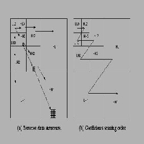
dinate symbol corresponding to a significant pixel and know-
IJSER © 2012
The research paper published by IJSER journal is about MEDICAL IMAGE COMPRESSION USING REGION GROWING SEGMENATION 5
ISSN 2229-5518
ing the threshold, the decoder is able to determine the range in which the pixel lies and reconstructs the pixel value to the midpoint of that range. Thus from the decoders viewpoint the rough estimate of a significant pixel's value is getting more refined and accurate as more subordinate passes are made. So, the subordinate passes quantize pixel values to a two symbol alphabet which then get encoded by using an adaptive arith- metic coder as described by Witten, Neal, and Cleary, thus achieving compression.
What is needed for decoding an image compressed by Shapi- ro's algorithm is the initial threshold, the original image size, the subband decomposition scale and, of course, the encoded bit stream. The decoder then decompresses the arithmetically encoded files into symbol files, creates all the proper size sub- bands needed since it knows the subband decomposition scale and the original image size, and proceeds to undo the Shapiro compression since it knows the initial threshold and the sub- band scanning order.
We use a two scale wavelet image as a simple to show the al- gorithm. The original image is shown in Figure.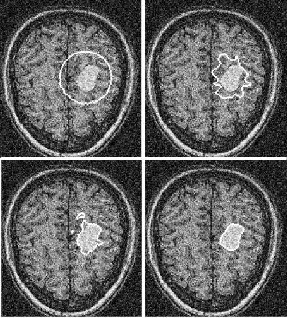
In this paper we used the seeded region growing algorithm for segmentation for segmenting the medical image and EZW for compression method and the compression ratio is high and the segmentation
[3] A. Abu-Hajar and R. Shankar, ‚Enhanced Partial-EZW for
Lossless Image Compression‛ Acoustics, Speech and
Signal processing 2003, Proceedings (ICASSP ’03)
*9+ Park, K., and Park, H.W.: ‘Region-of-interest coding based
on
set partitioning in hierarchical trees’, IEEE Trans. Circuits Syst. Video Technol., 2002, 12, (2), pp. 106–11
[3] Yian-Leng Chang, Xiaobo Li, ‚Adaptive image
region-growing‛, IEEE Transactions on Image
Processing, vol.3, no.6, Nov. 1994, pp.868-72.
*4+ Rolf Adams and Leanne Bischof, ‚Seeded Region Growing‛, IEEE Transactions on Image processing, Vol.16, No.6, June, 1994, pp.641-47
*5+ Hojjatoleslami SA, Kittler J., ‚Region growing: a new approach‛, IEEE Transactions of Image Processing, vol.7, no.7, July 1998, pp.1079-84.![]()
IJSER © 2012