International Journal of Scientific & Engineering Research, Volume 5, Issue 9, September-2014 49

ISSN 2229-5518

Mathematical Analysis of Stiff and Non-Stiff Initial Value Problems of Ordinary Differential Equation Using Matlab

*D. Omale, P.B. Ojih, M.O. Ogwo

Abstract - Many important and complex systems from different fields of sciences are modeled using differential equations. Due to the complexity of these systems, analytical methods are often difficult or impossible to implement for such problems and so numerical methods are the way out. The advent of computer applications like MATLAB starting from the mid 20th century has made a drastic improvement in numerical solutions for differential equations. In this work, we present the solvers in MATLAB for obtaining numerical solution for initial value problems of ODEs – ode45, ode23, ode113, ode15s, ode23s, ode23t, ode23tb. Six problems are solved, three of which are stiff and three non-stiff using the relevant MATLAB solvers and the solutions are presented.

Index Terms – Advent of computer application, Analytic approach, Differential equation, Dynamic, Matlab, Matrix laboratory, Non- Stiff, Stiff,

………………………………………….♦…………………………………………

1. INTRODUCTION

The dynamic behavior of systems is an interesting and important subject of study for scientists, Marcel B. Finan. (2012). Mechanical systems involve time related change in position and speed, electric systems involve change in current and voltage with time as well as several other systems from fields like engineering, economics, social sciences, biology, business and so on. These systems involving change are represented mathematically using differential equations. Differential equations are equations involving the derivatives of a dependent variable with respect to one or two independent variables.
Differential equations can be classified as ordinary or partial. A differential equation is ordinary if the unknown function is dependent only on a single variable. If the unknown function is dependent on multiple independent variables and the equation involves its partial derivatives, then the equation is a partial differential equation. Marcel, (2012).
Differential equations are also classified according to their order. The order of a differential equation is the highest derivative in the equation. A differential equation that has the second derivative as the highest derivative is said to be of order 2. The highest power of the highest derivative in a differential equation is the degree of the equation.
In physics, Newton’s Second Law, Navier Stokes
Equations, Cauchy-Riemman Equations, Schrodinger
Equations are all well known differential equations. The Lotka-Voltera Equations, Verhulst Equations and Replicator dynamics in biology as well as the exogenous growth model and Malthusian growth model in Economics are all represented by differential equations.
The solution of a differential equation is a value of the dependent variable in the equation that satisfies the equation at all points of the solution domain. The solution of a differential equation at a point is the value of the dependent variable at that point. Solutions to differential equations can be categorized in three broad sections. The analytic approach of solution, the qualitative approach and the numerical approach.
The analytic approach seeks to provide an explicit solution to the differential equation. Many important equations are impossible to solve using this method. The qualitative approach does not provide explicit solutions; rather it uses geometry to provide an overview of the behavior of the model. The qualitative approach yields solutions in form of direction fields, solution curves and phase plots. This method may be used to validate an analytic or numeric result. The numerical method provides approximate values of the solutions to the differential equation. The numerical method starts with an initial value of the variable and then uses the equations to figure out the changes in this variable over a brief time and continues to compute approximations of the solutions until the end of the desired solution interval.

IJSER © 2014 http://www.ijser.org

International Journal of Scientific & Engineering Research, Volume 5, Issue 9, September-2014 50

ISSN 2229-5518

Differential equations along with a specified value of the unknown function at a given point in the domain of the solution are an Initial Value Problem. This specified value is the initial condition. In many important cases of differential equations, analytic solutions are difficult or impossible to obtain and time
consuming. Eric, (2013). Although numerical
solutions are approximations, the error of approximation is often acceptable and numerical solutions give birth to algorithms that are used to design computer simulated solutions.
A major development in the study of numerical methods is the introduction of modern computers for the calculation of functions in the mid 20th century. Wikipedia, (2014). Until this time, numerical methods often depended on hand interpolation in large printed
tables. These tables contained data such as interpolation points and function coefficients up to 16 decimal places or more and were used to obtain very good numerical estimates of functions. Although these same algorithms continue to be part of the base of software algorithms for obtaining numerical solutions, the way computer represents and processes numbers gives rise to inexact results from the programs. Inexactness arises for different reasons like the number of decimal places in which results are retrieved and the number of steps required to the final solution, nevertheless, the use of computers and computer applications in numerical methods has become an established part of general numerical analysis with the development of many numerical computing applications such as MATLAB, S-PLUS, LabView, FreeMat, Scilab, GNU Octave and their associated speed and performance in obtaining solutions.

2. OVERVIEW OF MATLAB

MATLAB which stands for Matrix Laboratory is a high-level language and interactive computer environment developed by MathWorks for numerical computation, visualization, and programming. Using MATLAB, you can analyze data, develop algorithms, and create models and applications. The language, tools, and built-in math functions enable you to explore multiple approaches and reach a solution faster than with spreadsheets or traditional programming languages, such as C/C++ or Java.
You can use MATLAB for a range of applications, including signal processing and communications, image and video processing, control systems, test and measurement, computational finance, and computational biology. More than a million engineers and scientists in industry and
academia use MATLAB, the language of technical computing.

3. STIFFNESS OF ORDINARY DIFFERENTIAL EQUATIONS

Stiff ordinary differential equations arise frequently in the study of chemical kinetics, electrical circuits, vibrations, control systems and so on. It is a difficult and important concept in the study of differential equations. Stiffness has no generally accepted definition but several attempts had been made at defining the concept. Some of the definitions are:
1. A stiff problem is one for which no solution component is unstable (no eigenvalue of the Jacobian matrix has a real part which is at all large and positive) and at least some component is very stable (at least one eigenvalue has a real part which is large and negative.
2. A problem is stiff if the solution being sought varies slowly but there are nearby solutions that vary rapidly, so the numerical method must take small steps to obtain satisfactory results.
3. Stiffness occurs when some components decay more rapidly than others.
4. The linear system of differential equations

𝑑𝑢
= 𝑨𝑢(𝑡) 𝑡 ∈ [0, 𝑇]
𝑑𝑡
𝑢(0) = 𝑢0
is stiff when the eigenvalues 𝜆𝑘 (𝑘 = 1,2, … , 𝑚) of
the constant coefficient matrix 𝑨 of the system have
the following properties:
5. Re𝜆𝑘 < 0 for each 𝑘 = 1,2, … , 𝑚 (all its eigenvalues have negative real parts.

The number, 𝑆 defined as, 𝑆 = 𝑚𝑎𝑥𝑘 |𝑅𝑒𝜆𝑘| is large, i.e.

𝑚𝑖𝑛𝑘|𝑅𝑒 𝜆𝑘|

𝑆 ≫ 1. 𝑆 is called the stiffness number.
6. A problem is stiff if explicit methods fail to provide
solutions or works extremely slowly.
According to Shampine and Thompson as reported in Aliyu et al (2014), the best way to detect stiffness is to try one of the solvers intended for non- stiff systems. If it is unsatisfactory, then the problem may be stiff and effective stiff solvers should be employed. We shall employ this method of detecting stiffness in this work.
The objective of this work is to present how MATLAB solvers are applied in providing numerical solutions for initial value problems of ordinary differential equations.

IJSER © 2014 http://www.ijser.org

International Journal of Scientific & Engineering Research, Volume 5, Issue 9, September-2014 51

ISSN 2229-5518

4. MATLAB ODE SOLVERS

There are several inbuilt solvers for differential equations in MATLAB. Eight (8) of these solvers are applicable for initial value ODE problems. They are: ode45, ode23, ode113, ode15s, ode23s, ode23t, ode23tb, ode15i. These ODE solvers are designed to handle three types of first order ODEs:
1. Explicit ODEs of the form 𝑦 ′ = 𝑓(𝑡, 𝑦)
2. Linearly implicit ODEs of the form 𝑴(𝑡, 𝑦). 𝑦 ′ =
𝑓(𝑡, 𝑦), where 𝑴(𝑡, 𝑦) is a matrix.
3. Fully implicit ODEs of the form 𝑓(𝑡, 𝑦, 𝑦 ′) = 0
In this work, we shall consider explicit ODEs only.
Initial value problems are categorized as stiff and non-stiff, Shampine, et al (2003) and this classification is important in selecting the solvers to use in MATLAB. Stiffness is a subtle, complicated and important concept in numerical solutions of ordinary differential equations. A problem is stiff if the solution being sought varies slowly, but there are nearby solutions that vary rapidly and so the numerical method must take small steps to obtain satisfactory results. Stiffness also forms a basis for the classification of ODE solvers in MATLAB. Some solvers are designed for stiff problems and some others for non-stiff problems. Stiffness is an efficiency issue. If non-stiff methods are used to solve stiff IVPs, the solver will either take an extremely long time to supply a solution or supply an inaccurate solution or fail to supply any solution at all. All stiff problems are difficult for solvers that are not designed for them and this is why it is necessary to select an appropriate solver when using MATLAB ODE solvers. MATLAB documentation recommends that ode45 is the best solver to give the first try for most problems. If ode45 is slow in solving the problem or failed to solve the problem, then stiffness is suspected and you can then go ahead to try ode15s.

Ode45

ode45 is a sophisticated built-in MATLAB function that gives very accurate solutions. Ode45 is based on a simultaneous implementation of an explicit fourth and fifth order Runge-Kutta formula called the Dormand-Prince pair. It is a one-step solver. This is the first solver to be tried for most problems. It is designed for non-stiff problems. Ode45 can use long step size and so the default is to compute solution values at four points equally spaced within the span of each natural step.
The Dormand-Prince pair is an explicit method and a member of the Runge-Kutta family of solvers. The method employs function evaluations to calculate
fourth and fifth order accurate solutions. The difference between these solutions is then taken to be the error of the fourth order solution.

Ode23

This solver is designed for solving non-stiff problems. It’s method is based on the 2nd and 3rd Order Runge-Kutta pair called the Bogacki-Shampine method. Ode23 is less expensive than ode45 in that it requires less computation steps than ode45. But it is of a lower order, although it may be more efficient at crude tolerances and in the presence of mild stiffness. Ode23 is a one-step solver.
The Bogacki-Shampine method is a Runge-Kutta method of order 3 with four stages proposed by Przemyslaw Bogacki and Lawrence F. Shampine in
1989. It uses three function evaluations per step. It has embedded second order method which is used to implement adaptive step size for the method.

Ode113

Ode113 is a multi-step variable order method which uses Adams–Bashforth–Moulton predictor- correctors of order 1 to 13. It may be more efficient than ode45 at stringent tolerances and when the ODE problem is particularly expensive to evaluate. It is designed for non-stiff problems.

Ode 15s

Ode15s a variable order solver whose algorithm is based on the numerical differentiation formulas (NDFs) and optionally along with the backward differentiation formulas (BDFs) which is also called Gear’s method. This is a multi-step solver that is designed for stiff problems. This is the next recommended solver if ode45 fails or is too slow.
The Backward Differentiation Formula is a family of implicit methods for the numerical integration of ordinary differential equations. They are linear multi-step methods and for a given function and time, they approximate the derivative of that function using information from already computed times. BDF methods are implicit and, as such, require the solution of nonlinear equations at each step.

Ode23s

This is based on a modified Rosenbrock formula of order 3 and 2 with error control designed for stiff
systems. It advances from 𝑦𝑛 to 𝑦𝑛+1 with the second
order method and controls the local error by taking
the difference between the third and second order numerical solutions. This is a one step method and

IJSER © 2014 http://www.ijser.org

International Journal of Scientific & Engineering Research, Volume 5, Issue 9, September-2014 52

ISSN 2229-5518

can solve some kinds of stiff problems for which ode15s is not effective.

Ode23t

The algorithm implemented in this solver is the trapezoidal rule along with a free interpolant. This solver is designed for only moderately stiff problems and when the solution required should be without damping.

Ode23tb

Is an implementation of TR-Backward Differentiation Formula 2. This is an implicit Runge- Kutta formula with a first stage that is a trapezoidal rule step and a second stage that is a backward differentiation formula of order 2. This method may
be used when crude error tolerance is required to solve stiff systems.

Ode15i

This solver is designed based on a variable order method for fully implicit differential equations. This is the only solver that is designed for fully implicit differential equations.

A Summary of MATLAB ODE Solvers

5. MATLAB ODE SOLVER SYNTAX

Apart from the ode15i solver, all other ODE solvers in MATLAB have the same syntax. This makes it easy to apply different methods to the same problem. The basic syntax for all the solvers is
[𝑡, 𝑦] = 𝑠𝑜𝑙𝑣𝑒𝑟(𝑓, 𝑡𝑠𝑝𝑎𝑛, 𝑦0, 𝑜𝑝𝑡𝑖𝑜𝑛𝑠)
Where 𝑠𝑜𝑙𝑣𝑒𝑟 is the ode solver method, e.g. ode45,
ode23 and others.
The output arguments are:

The input arguments are:

6. Optional Parameters.

The default integration properties for the ODE
solvers are selected to handle common problems. It is
possible to use optional parameters to improve ODE
solvers performance. This will override the default integration properties of the solver.
The optional properties that can be set are in several categories. Some of them are Error Control Properties, Solver Output Properties, Step-Size Properties, Event Location Property, Jacobian Matrix Properties.
On the error control properties, each MATLAB ODE solver is designed in a manner that the estimated local error in each component of the solution satisfies a given error test. For a single equation the estimated
local error in passing from 𝑦(𝑡𝑛 ) to 𝑦(𝑡𝑛+1 ), call it
𝑒(𝑡𝑛 ), is to satisfy |𝑒(𝑡𝑛 )| ≤ 𝑚𝑎𝑥{𝐴𝑏𝑠𝑇𝑜𝑙, 𝑅𝑒𝑙𝑇𝑜𝑙 ·
|𝑦(𝑡𝑛 )|}. The error tolerances 𝐴𝑏𝑠𝑇𝑜𝑙 and 𝑅𝑒𝑙𝑇𝑜𝑙 can
be specified by running the MATLAB program
𝑜𝑑𝑒𝑠𝑒𝑡; when left unspecified, the default tolerances
are 𝐴𝑏𝑠𝑇𝑜𝑙 = 10−6, 𝑅𝑒𝑙𝑇𝑜𝑙 = 10−3 .
The step size properties specify the size of the
first step the solver should use and the upper bound on the step size that the solver can use. The property
that specifies the initial step size is called 𝐼𝑛𝑖𝑡𝑖𝑎𝑙𝑆𝑡𝑒𝑝

IJSER © 2014 http://www.ijser.org

International Journal of Scientific & Engineering Research, Volume 5, Issue 9, September-2014 53

ISSN 2229-5518

and the property that specifies the upper bound on
solver step size is called 𝑀𝑎𝑥𝑆𝑡𝑒𝑝. To set optional parameter properties, we use the 𝑜𝑑𝑒𝑠𝑒𝑡 function and
the syntax is as shown below:
𝑜𝑝𝑡𝑖𝑜𝑛𝑠
= 𝑜𝑑𝑒𝑠𝑒𝑡(‘𝑛𝑎𝑚𝑒1’, 𝑣𝑎𝑙𝑢𝑒1, ‘𝑛𝑎𝑚𝑒2’, 𝑣𝑎𝑙𝑢𝑒 2, … )
‘name1’ refers to the property name that has the
specified value ‘value1’. Any property that is unspecified retains its default value.
For example, to set the initial step size, we have
𝑜𝑝𝑡𝑖𝑜𝑛𝑠 = 𝑜𝑑𝑒𝑠𝑒𝑡(′𝐼𝑛𝑖𝑡𝑖𝑎𝑙𝑆𝑡𝑒𝑝′ , 0.0001)

7. PROCEDURE FOR SOLVING FIRST ORDER

PROCEDURE FOR SOLVING HIGHER ORDER ODEs USING MATLAB SOLVERS

1. Rewrite the second order ODE as a system of first order ODEs.

For the nth-order ODE: 𝑦 (𝑛) = 𝑓�𝑡, 𝑦, 𝑦 ′ , … , 𝑦 (𝑛−1) �
Set 𝑦1 = 𝑦, 𝑦2 = 𝑦 ′ , … , 𝑦𝑛 = 𝑦 (𝑛−1)
The result of this substitution will be an equivalent
system of 𝑛 first order ODEs

′ = 𝑦

𝑦1 2

′ = 𝑦

𝑦2 3
⋮
𝑦 ′ = 𝑓(𝑡, 𝑦 , 𝑦 , … , 𝑦 )

𝑛 1 2 𝑛

For example, consider the second order ODE
𝑦 ′′ = 𝑓(𝑡, 𝑦, 𝑦 ′ )
Set, 𝑦1 = 𝑦 and 𝑦2 = 𝑦′

′ = 𝑦 ′ = 𝑦

and 𝑦 ′ = 𝑦 ′′ =

ODEs USING MATLAB SOLVERS

1. Code the Problem

In this step, you develop an m-file to contain the
given function. For the general problem of the form
𝑦 ′ = 𝑓(𝑡, 𝑦), the code will look like this:
𝑓𝑢𝑛𝑐𝑡𝑖𝑜𝑛 𝑑𝑦𝑑𝑡 = 𝑝1(𝑡, 𝑦)
𝑑𝑦𝑑𝑡 = 𝑓(𝑡, 𝑦);
𝑒𝑛𝑑
For example, consider the problem, 𝑦′ = 2𝑡 + 1, the
code for the problem is:
𝑓𝑢𝑛𝑐𝑡𝑖𝑜𝑛 𝑑𝑦𝑑𝑡 = 𝑝1(𝑡, 𝑦)
𝑑𝑦𝑑𝑡 = 2 ∗ 𝑡 + 1;
𝑒𝑛𝑑
The names 𝑑𝑦𝑑𝑡 𝑎𝑛𝑑 𝑝1 in the code above do not
play any role in the definition of the function. Any
name can be used as long as they conform with
MATLAB naming rules for functions and m-files.

2. Apply a Solver to the Problem

Make a decision of the solver you intend to use. Then
call the solver using the syntax in Section 3.4.1 and pass the function, the time interval you desire for your solution and the initial condition vector to it. For example, to apply ode45 solver to the problem
described by 𝑝1 in step 1 above on the time interval between 0 and 10, with initial condition 𝑦(0) = 0, the
following code is typed into the command window:
𝑡𝑠𝑝𝑎𝑛 = [0, 10];
𝑦0 = 0
[𝑡, 𝑦] = 𝑜𝑑𝑒45(@𝑝1, 𝑡𝑠𝑝𝑎𝑛, 𝑦0)

3. Retrieve the Solver Output

You can simply use the 𝑝𝑙𝑜𝑡 command to view the solver output. i.e. 𝑝𝑙𝑜𝑡(𝑡, 𝑦)
You can also display the results by using the
𝑑𝑖𝑠𝑝 command i.e. 𝑑𝑖𝑠𝑝([𝑡, 𝑦])
Phase portrait of the solution can also be retrieved.
This implies that, 𝑦1 2 2
𝑓(𝑡, 𝑦1 , 𝑦2)
So, we obtain the system of first order ODEs,
𝑦 ′ = 𝑦
𝑦 ′ = 𝑓(𝑡, 𝑦 , 𝑦 )

2. Code the system of First Order ODEs.

Develop an m-file containing the system of first order
ODEs obtained from splitting the higher order ODE
in question. For the general second order ODE in step
1 above, the code will look like this:
𝑓𝑢𝑛𝑐𝑡𝑖𝑜𝑛 𝑑𝑦𝑑𝑡 = 𝑝2(𝑡, 𝑦)
𝑑𝑦𝑑𝑡(1) = 𝑦(2);
𝑑𝑦𝑑𝑡(2) = 𝑓(𝑡, 𝑦1 , 𝑦2);
𝑑𝑦𝑑𝑡 = [𝑑𝑦𝑑𝑡(1); 𝑑𝑦𝑑𝑡(2)];
𝑒𝑛𝑑

3. Apply a Solver to the Problem.

You use the solver syntax to call the solver you want
to use as in the case of the first order ODE.

4. Retrieve the Solver Output

You can simply use the 𝑝𝑙𝑜𝑡 command to view the solver output. i.e. 𝑝𝑙𝑜𝑡(𝑡, 𝑦)
You can also display the results by using the
𝑑𝑖𝑠𝑝 command i.e. 𝑑𝑖𝑠𝑝([𝑡, 𝑦])
Phase portrait of the solution can also be retrieved.

APPLICATION OF MATLAB ODE SOLVERS TO NON-STIFF INITIAL VALUE PROBLEMS OF ODEs.

In this section, we apply the relevant solvers to three non-stiff problems (Problems 1, 2 and 3) and three stiff problems (Problems 4, 5 and 6). Solution graphs and Phase Portraits of the systems are also presented.

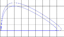
Problem 1:

IJSER © 2014 http://www.ijser.org

International Journal of Scientific & Engineering Research, Volume 5, Issue 9, September-2014 54

ISSN 2229-5518

The state variable equations of a continuous system describing the dynamic behaviour of the system is given by
𝑦1 = 5𝑦2
𝑦2 ’ = −𝑑𝑦2 + 𝑐𝑦1 𝑦2
due to Lotka and Volterra.
The parameters 𝑏 and 𝑑 govern the birth rate of prey and death rate of predators, respectively, and the
𝑦 ′ = −5𝑦 − 5𝑦 + 5
𝑦1 (0) = 𝑦2(0) = 0
Develop a MATLAB program that plots 𝑦1 𝑎𝑛𝑑 𝑦2 on
the same graph for 𝑡 = 0 𝑡𝑜 10. obtain the phase
portrait of the system.
Source: Exercises from Ogbonnaya (2008)

Solution: Using ode45 to solve the problem:

parameter 𝑐 governs the interaction of the two populations. With the parameter values 𝑏 = 1, 𝑑 =
10, and 𝑐 = 1, and initial conditions 𝑦1 (0) = 0.5
and 𝑦2(0) = 1
(the populations are normalized, and we treat them as
continuous variables), use MATLAB function ode45 to solve this system numerically, integrating to
𝑡 = 10. Plot each of the two populations as a
function of time, and on a separate graph plot the
trajectory of the point (𝑦1 (𝑡), 𝑦2 (𝑡)) in the plane.

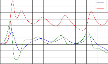
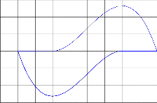
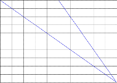
1.2

1

0.8

0.6

PLOT OF y1 AND y2 AGAINST t

y1 y2

Source: Heath (1997)

Solution:

Our system of ODEs now become

0.4

0.2

𝑦 ′
= 𝑦1 – 𝑦1 𝑦2

0

-0.2

0 1 2 3 4 5 6 7 8 9 10

t

𝑦2’ = −10𝑦2 + 𝑦1 𝑦2
𝑦1 (0) = 0.5 , 𝑦2 (0) = 1
Implementing ode45 for the problem:

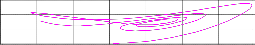
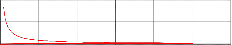
Phase Portrait of the System

PLOT OF PREY AND PREDATOR POPULATION AGAINST t

45

Prey

40 Predator

35

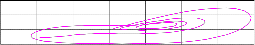
0.6

0.5

0.4

0.3

0.2

0.1

0

-0.1

GRAPH OF y2 AGAINST y1

0 0.2 0.4 0.6 0.8 1 1.2 1.4 y1

30

25

20

15

10

5

0

-5

0 2 4 6 8 10

t

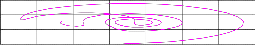
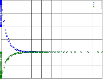
Phase Portrait of the System

PLOT OF PREDATOR POPULATION AGAINST PREY POPULATION

25

20

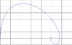
Problem 2.

Lotka-Volterra Equations

The populations of two species, a prey denoted by 𝑦1
and predator denoted by 𝑦2, can be modeled by a
system of ODEs:

15

10

5

0

-5

0 5 10 15 20 25 30 35 40 45

Prey

𝑦 ′
= 𝑏𝑦1 – 𝑐𝑦1 𝑦2

Problem 3:

IJSER © 2014 http://www.ijser.org

International Journal of Scientific & Engineering Research, Volume 5, Issue 9, September-2014 55

ISSN 2229-5518

Lorentz Equations

The Lorentz equations are used to simulate the

𝑑𝑦
𝑑𝑡
= 75𝑥 − 𝑦 − 𝑥𝑧
convection of a layer of fluid of infinite horizontal extent heated from below. The model is a simplified version of the heating of the atmosphere. The equations are obtained by expanding the terms for temperature and pressure involved in the problem with their Fourier series expansion and simplifying the expansion to the first three modes represented by the variables x, y, and z. The resulting system of equations is

𝑑𝑧
= 𝑥𝑦 – 2.666𝑧
𝑑𝑡
𝑥(0) = 1, 𝑦(0) = 1, 𝑧(0) = 1
Solving the problem using ode45:

PLOT OF x, y, z AGAINST t

𝑑𝑥
𝑑𝑡
= 𝜎 (−𝑥 + 𝑦)

140

x

120 y z

100

80

𝑑𝑦
𝑑𝑡

60

= 𝑟𝑥 − 𝑦 − 𝑥𝑧

0

where

𝑑𝑧
𝑑𝑡
= 𝑥𝑦 − 𝑏𝑧

-20

-40

-60

0 0.2 0.4 0.6 0.8 1 1.2 1.4 1.6 1.8 2 t

𝜎 , 𝑟, and 𝑏 are constants that result from combining physical parameters of the problem. Solve the Lorentz
equations for the following combination of parameters:
𝜎 = 10, 𝑟 = 75, 𝑏 = 2.666, 𝑥(0) = 1, 𝑦(0)
= 1, 𝑧(0) = 1
Plot the signals 𝑥 − 𝑣𝑠 − 𝑡, 𝑦 − 𝑣𝑠 − 𝑡, 𝑧 − 𝑣𝑠 − 𝑡, as
well as the phase portraits 𝑥 − 𝑣𝑠 − 𝑦, 𝑥 − 𝑣𝑠 − 𝑧,
and 𝑦 − 𝑣𝑠 − 𝑧.
Source: Gilberto (2004)

Solution:

Our system of ODEs now become:

Phase Portraits of the System

100

50

0

-50

-30 -20 -10 0 10 20 30 40

y

150

100

50

0

-30 -20 -10 0 10 20 30 40

z

150

100

50

0

-60 -40 -20 0 20 40 60 80

z

𝑑𝑥
𝑑𝑡
= 10(−𝑥 + 𝑦)

Comparison of ode45, ode23 and ode113 for Problems 1, 2, and 3

IJSER © 2014 http://www.ijser.org

International Journal of Scientific & Engineering Research, Volume 5, Issue 9, September-2014 56

ISSN 2229-5518

APPLICATION OF MATLAB ODE SOLVERS TO STIFF INITIAL VALUE PROBLEMS OF ODEs.

Problem 4.

1500

1000

500

0

Phase Plot for Van der Pol System

Van der Pol System

The Van der Pol system is a non-linear oscillator. This is a classical stiff problem in the field of electrical engineering and was first reported in 1927 by Balthazar Van der Pol and his colleague Van der Mark. The mathematical representation of the system is:
𝑦 ′ = 𝑦

′ 2

-500

-1000

-1500

-2.5 -2 -1.5 -1 -0.5 0 0.5 1 1.5 2

y1

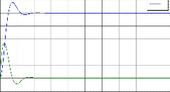
Problem 5:

The Robertson’s Problem
Consider the system below on the interval 0 ≤ 𝑡 ≤
5000
𝑦2 = 𝛼(1 − 𝑦1 )𝑦2 − 𝑦1

′ 4

The stiffness can be controlled by changing the
parameter 𝛼. 𝛼 = 1000 will result in a stiff case. We
shall solve the system with the initial conditions
𝑦1 = −.04𝑦1 + 10 𝑦2 𝑦3
𝑦 ′ = .04𝑦 − 104 𝑦 𝑦 − 3.107 𝑦2

2 1 2 3 2

′ 7 2

𝑦1 (0) = 2 and 𝑦2(0) = 0 on the interval 0 to 3000.
Source: Yihai (2000)

Solution

Our system of ODEs now become:
𝑦 ′ = 𝑦
𝑦3 = 3.10 𝑦2
𝑦1 (0) = 1, 𝑦2 (0) = 0, 𝑦3(0) = 0

′ 2

𝑦2 = 1000(1 − 𝑦1 )𝑦2 − 𝑦1
𝑦1 (0) = 2, 𝑦2 (0) = 0
Solving with ode15s:

Solution:

Solving with ode15s:

2

1.5

1

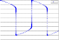
PLOT OF VAN DER POL SYSTEM

y1

1

0.9

0.8

PLOT OF y1, y2 and y3 AGAINST t

y1 y2 y3

0.5

0.7

0 0.6

-0.5

0.5

-1

-1.5

0.4

0.3

0.2

-2

-2.5

0 500 1000 1500 2000 2500 3000 t

0.1

0

0 500 1000 1500 2000 2500 3000 3500 4000 4500 5000 t

Phase Portrait of the System

Phase Portraits of the System

IJSER © 2014 http://www.ijser.org

International Journal of Scientific & Engineering Research, Volume 5, Issue 9, September-2014 57

ISSN 2229-5518

-3

x 10

3

2

1

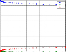
Solution: Solving with ode15s

0

0.91 0.92 0.93 0.94 0.95 0.96 0.97 0.98 0.99 1

y1

0.1

0.05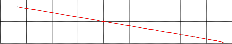

0

0.91 0.92 0.93 0.94 0.95 0.96 0.97 0.98 0.99 1

y1

0.1

0.05

2

1.5

1

0.5

0

PLOT OF y1 and y2 AGAINST t

y1 y2

0

0 0.5 1 1.5 2 2.5 3

-0.5

y2 x 10-3

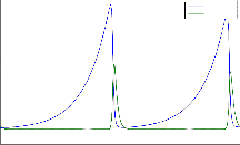
Problem 6

-1

0 2 4 6 8 10 12 14 16 18 20

t

Consider the system of stiff differential equations on
the interval 0 ≤ 𝑡 ≤ 20
𝑦 ; = 998𝑦 + 1998𝑦
𝑦 ′ = −999𝑦 − 1999𝑦
𝑦1(0) = 1, 𝑦2 (0) = 0

0

-0.1

-0.2

-0.3

-0.4

-0.5

-0.6

-0.7

-0.8

-0.9

-1

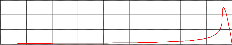
Phase Portrait of the Solution

PLOT OF y1 AGAINST y2

0 0.2 0.4 0.6 0.8 1 1.2 1.4 1.6 1.8 2 y1

Comparison of ode15s, ode23s and ode23t for Problems 4, 5, and 6

CONCLUSION

IJSER © 2014 http://www.ijser.org

International Journal of Scientific & Engineering Research, Volume 5, Issue 9, September-2014 58

ISSN 2229-5518

The use of MATLAB is very effective in proffering numerical solution to initial value problems of ordinary differential equations as seen in this work. Calculations that could run through pages and days are obtained in a matter of seconds. Accuracy is also maintained. Further studies on the use of optional
parameters to enhance performance of solvers is
recommended.

REFERENCES

Aliyu B. K., Osheku C. A., Funmilayo A. A. and Musa J.I. (2014) Identifying Stiff Ordinary Differential Equations and Problem Solving Environments (PSEs). Journal of Scientific Research

& Reports. 3(11): 1430 - 1448

Bilokon P., Amen S., Brinley Codd A., Fofaria M., Shah T. (2004). Numerical Solutions of Differential Equations. Retrieved March 3, 2014 from www.oc.ic.ac.uk/~pb401/DE/archive/report/report.pdf
Butcher J.C. (2000) Numerical Methods for Ordinary Differential Equations in the 20th Century. Journal of Computational and Applied Mathematics 125:1-29
Coddington Earl A. and Levinson Norman (1955) Theory of Ordinary Differential Equation. (London, McGraw-Hill Book Company, Inc.)
David Houcque. (2014). Applications of MATLAB: Ordinary Differential Equations (ODE). Retrieved March 30, 2014 from www.math.unipd.it/~alvise/CS_2008/ODE/MFILES/ ode.pdf
Didier Gonze. (2013). Numerical Methods for

Ordinary Differential Equations. Retrieved March 10,

2014 from http://homepages.ulb.ac.be/~dgonze/TEACHING/nu merics.pdf
Gilberto E. Urroz. (2004). Examples of Initial-Value ODE Problems. Retrieved April 5, 2014 from ocw.usu.edu/Civil_and_Environmental_Engineering/ Numerical_Methods_in_Civil
_Engineering/ODEsExamples.pdf
James Blanchard. (1998). Ordinary Differential

Equations: Initial Value Problems. Retrieved March

19, 2014 from http://homepages.cae.wisc.edu/~blanchar/eps/ivp/ivp. html
Kendall Atkinson, Weimin Han, David Stewart (2009) Numerical Solutions of Ordinary Differential Equations. (New Jersey, John Wiley & Sons, Inc.)
Shampine L. F., Gladwell I., Thompson S. (2003) Solving ODEs in MATLAB. (New York, Cambridge University Press)
Marcel B. Finan. (2012). A first Course in Elementary Differential Equations. Retrieved March 30, 2014 from www.math.umass.edu/~gardner/m331/diffq1book.pdf
Mathworks. (2014). MATLAB, The Language of Technical Computing. Retrieved April 3, 2014 from http://www.mathworks.com/products/matlab/index.ht ml?sec=applications
Ogbonnaya, I. O. (2008) Introduction to MATLAB/SIMULUNK for Engineers and Scientists. (Enugu, John Jacob’s Classic Publishers Ltd.)
Ogunride R. Bosede, Fadugba S. Emmanuel, Okunlola J. Temitayo (2012) On Some Numerical Methods For Solving Initial Value Problems In Ordinary Differential Equations. IOSR Journal of Mathematics. 1(3):25-31
Paul’s Online Math Notes. (2014). Differential Equations-Notes. Retrieved March 13, 2014 from tutorial.math.lamar.edu/Classes/DE/Definitions.aspx
Yihai Yu. (2000) Stiff Problems in Numerical Simulation of Biochemical and Gene Regulatory Networks. Retrieved April 5, 2014
From www.getd.libs.uga.edu/pdfs/yu_yihai_200408_ms.pdf
Robert E. Terrell (2014). Lecture Note on Differential Equations. Retrieved March 9, 2014 from http://www.math.cornell.edu/~bterrell/dn.pdf
Ryuichi Ashino, Michihiro Nagae and Remi Vaillancourt (2000) Behind and Beyond MATLAB ODE Suite. Computers and Mathematics with Applications. 40:491-512
Sharaban Thohura & Azad Rahman (2013) Numerical Approach for Solving Stiff Differential Equations: A Comparative Study. Global Journal of Science Frontier Research Mathematics and Decision Sciences. 13(6): 6 - 18

IJSER © 2014 http://www.ijser.org

International Journal of Scientific & Engineering Research, Volume 5, Issue 9, September-2014 59

ISSN 2229-5518

Steven T. Karris (2007) Numerical Analysis Using MATLAB and Excel (California: Orchard Publications)
Toshinori Kimura. (2009). On Dormand-Prince Method. Retrieved April 27, 2014 from http://depa.fquim.unam.mx/amyd/archivero/ DormandPrince_19856.pdf
Wikipedia. (2014). Bogacki Shampine Method. Retrieved April 27, 2014 from http://en.wikipedia.org/w/index.php?title=Bogacki- Shampine_method
Wikipedia. (2014). Differential Equation. Retrieved February 20, 2014 from http://en.wikipedia.org/wiki/Differential_equation

http://en.wikiboos.org/wiki/MATLAB_Programming
http://en.wikipedia.org/wiki/Initial_Value_Problem

IJSER © 2014 http://www.ijser.org