International Journal of Scientific & Engineering Research Volume 2, Issue 5, May-2011 1

ISSN 2229-5518

Load Forecasting Using New Error Measures

In Neural Networks

Devesh Pratap Singh, Mohd. Shiblee, Deepak Kumar Singh

Abstract— Load forecasting plays a key role in helping an electric utility to make important decisions on power, load switching, voltage control, network reconfiguration, and infrastructure development. It enhances the energy-efficient and reliable operation of a power system. This paper presents a study of short-term load forecasting using new error metrices for Artificial Neural Networks (ANNs) and applied it on the England ISO.

Index Terms— Load forecasting, Neural networks, New neuron Models, New error metrics for neural networks, England ISO

—————————— • ——————————

1 INTRODUCTION

here is a growing tendency towards unbundling the electricity system. This is continually confronting the different sectors of the industry (generation, trans- mission, and distribution) with increasing demand on planning management and operations of the network. The operation and planning of a power utility company requires an adequate model for electric power load fore- casting. Load forecasting plays a key role in helping an electric utility to make important decisions on power, load switching, voltage control, network reconfiguration,

and infrastructure development.

Methodologies of load forecasts can be divided into

various categories that include short-term forecasts, me-

dium-term forecasts, and long-term forecasts. Short-term

forecasting which forms the focus of this paper, gives a

forecast of electric load one hour ahead of time. Such

forecast can help to make decisions aimed at preventing

imbalance in the power generation and load demand,

thus leading to greater network reliability and power

quality.

Many methods have been used for load forecasting in

the past. These include statistical methods such as regres- sion and similar-day approach, fuzzy logic, expert sys- tems, support vector machines, econometric models, end- use models, etc. [2].

A supervised artificial neural network has been used in this work. Here, the neural network is trained on input data as well as the associated target values. The trained network can then make predictions based on the relation- ships learned during training. A real life case study of the power industry in Nigeria was used in this work.

In this paper a supervised artificial neural network has been used for load forecasting.

• Devesh Pratap Singh is a graduate in engineering from UP Technic- al University, India. E-mail: deveshpratap.85@gmail.com

• Mohd. Shiblee is currently pursuing PhD from IIT Kanpur, India, E-mail: shiblee@iitk.ac.in

• Deepak Kumar Singh is currently pursuing PhD from IIT Kanpur,

India, E-mail: deepaks@iitk.ac.in

Here, the neural network is trained on input data as well as the associated target values. The error measures used in the presented model is different from the conventional models. England ISO data has been used for the simula- tion.

In further sections of this paper, we discuss neural net- work in greater detail, introduce the conventional model of artificial neural network and the mathematical error models used in our model.

2 NEURAL NETWORK

2.1 INTRODUCTION

Artificial neuron model is inspired by biological neu- ron. Biological neurons are the basic unit of brain for in- formation processing system. Artificial Neural Network is a massive parallel distributed processing system that has a natural propensity for storing experimental know- ledge and making it available for use [1]. The basic processing units in ANN are neurons. Artificial Neural Network can be divided in two categories viz. Feed- forward and Recurrent networks. In Feed-forward neural networks, data flows from input to output units in a feed- forward direction and no feedback connections are present in the network. Widely known feed-forward neural networks are Multilayer Perceptron (MLP) [3], Probabilistic Neural Network (PNN) [4], General Regres- sion Neural Network (GRNN) [5] and Radial Basis Func- tion (RBF) Neural Networks [6]. Multilayer Perceptron (MLP) is composed of a hierarchy of processing units (Perceptron), organized in series of two or more mutually exclusive sets layers. It consists of an input layer, which serves as the holding site for the input applied to the network. One or more hidden layers with desired number of neurons and an output layer at which the overall map- ping of the network input is available [7]. There are three types of learning in Artificial Neural Networks, Super- vised, unsupervised and Reinforcement learning. In su- pervised learning, the network is trained by providing it with input and target output patterns. In Unsupervised

International Journal of Scientific & Engineering Research Volume 2, Issue 5, May-2011 2

ISSN 2229-5518

learning or Self-organization, an (output) unit is trained to respond to clusters of pattern within the input. In this paradigm the system is supposed to discover statistically salient features of the input population.Reinforcement learning may be considered as an intermediate form of supervised and unsupervised learning. Here the learning machine does some action on the environment and gets a feedback response from the environment. Most popular learning algorithm for feed-forward networks is Back- propagation. The first order optimization techniques in Back-propagation which uses steepest gradient decent algorithm show poor convergence. ANN is a very popu- lar tool in the field of engineering. It has been applied for various problem like times series prediction, classifica- tion, optimization, function approximation, control sys- tems and vector quantization. Many real life application fall into one of these categories. In the existing literature, various neural network learning algorithms have been used for these applications. In this paper, MLP neural network has been used successfully with different error measures for load forecasting.

2.2 New Error Measures

In Back-propagation algorithm, training of the neuron model is done by minimizing the error between target value and the observed value. In order to determine error between target and observed value, distance metric is used. It has been observed that Euclidean distance metric is the most commonly used for error measures in Neural Network applications. But it has been suggested that this distance metric is not appropriate for many problems [12]. In this work the aim is to find best error metric to use in Back propagation learning algorithm.
The likelihood and log-likelihood functions are the ba-
sis for deriving estimators for parameters, for given set of data. In maximum likelihood method we estimate the value of “y” for the given value of “x” in presence of er- ror. (See equation (1))
be used to improve the performance of the neuron model for learning the best-fit weights of the neuron models. Distance metrics associated with the distribution models that imply the arithmetic mean, harmonic mean and geometric mean in (See Table 1) are inferred using equa- tion (3).
TABLE 1

ERROR METRICS AND MEAN ESTIMATION

	Error metric	Mean
Arithmetic	N 2 E = ( xi , J. ) i =1	N J.0 = 1 x i N i = 1
Harmonic	2 N ( J. E = xi 1 I = 0 i =1 xt )	N J.0 = N 1 x i = 1 i
Geometric	2 N l ( x i l E = l og I = 0 i = 1 L J.0 ) J	1 ( N N J.0 = n x 1 I i = 1 )

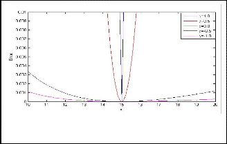
Fig. 1.the error criterion of the arithmetic mean, harmonic and geometric mean

Figure 1 illustrates the difference between the distance (error) metrics for the arithmetic mean, harmonic mean and geometric mean. For the sake of comparison, the val-

y i = xi + e

(1)

ue of µ is set to 15. It is found that in the distribution as-
Let xi denote the data points in the distribution and let N
sociated with the harmonic and geometric estimations,
denotes the number of data points. Then an estimator

the observations xi which are far away from

J.0

will con-
of µ can be estimated by minimizing the error metric with respect to J.

tribute less towards µ, in contrast to arithmetic mean and
thus the estimated values will be less sensitive to the bad observations (i.e., observation with large variance), and

E = f ( x, J. )

i =1

where f ( x, J. )

(2)

is the distance metric. The error function E
therefore they are more robust in nature [9].

.Due to the robust property of harmonic and geometric distance metrics, generalizations of these distance metrics

is differentiated with respect to J. and equated to zero.
have also been done which may fit the distribution of da-
ta better [8-9]

E N

= f ( x, J. ) = 0

(3)

2.2.1 Generalized Harmonic Type I Error Metric

i =1 J.

Generalized Harmonic Type I Error metric derived from
Jie, et. al., [10-11] has proposed some new distance me-
trics based on different means. These distance metrics can
the Generalized Harmonic Type I mean estimation using

International Journal of Scientific & Engineering Research Volume 2, Issue 5, May-2011 3

ISSN 2229-5518

equation (3) is given below.
Generalized Harmonic Type I Mean:
distance metric for the generalized harmonic mean Type
II

N p 1

( x I

)

(4)

0J.

= i = 1

i = 1

p 2

( x I

)

The corresponding error metric is given below: Generalized Harmonic Type I Error Metric:

N (0J.

(5)

E =

i = 1

( x i ) 1 I

i )

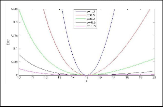
The parameter ‘p’ is used to define the specific distance metrics. If p=1, it becomes ordinary harmonic distance metric and for p=2, it will become Euclidean distance me- tric. Figure 2 illustrates the generalized harmonic Type I distance metric for the Generalized Harmonic Mean Type I.

Fig. 3: The error criterion of the Generalized Harmonic Mean

Type II

2.2.3 Generalized Geometric Error Metric

Generalized Geometric Error Metric derived from the Generalized Geometric Mean estimation using equation (3) is given below

. Generalized Geometric Mean:

0J. = l n

( x )( x i ) l

i = 1

( x i )

L i = 1 J (8

The corresponding error metric is given below: Generalized Geometric Error Metrics :

N l

E = (x )r log

( xi l

(9)

i =1 L

J. )J

Fig. 2: The error criterion of the Generalized Harmonic Mean

Type 1

2.2.2 Generalized HarmonicType II Error metric

Harmonic Type II Error metric derived from the Genera- lized Harmonic Type II mean estimation using equation (3) is given below.
GeneralizedHarmonicType II Mean:

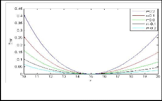
The parameter ‘r ’ is used to define the specific distance metrics. For the generalized geometric mean estimation, if r = 0, it will become an ordinary geometric mean. Figure
4 illustrates the generalized geometric distance metric for the generalized geometric mean.

l l q

0J. = N

L i = 1

( x i )

(6)

Generalized Harmonic Type II Error Metric:

E = l( x ) q

( J.0 ) q l

(7)

Fig. 4: The error criterion of the Generalized Geometric Mean

L i J

i =1

The parameter q is used to define the specific distance metrics. If q= -1, it becomes ordinary harmonic distance metric and for q=1, it will become Euclidean distance me- tric. Figure 3 illustrates the generalized harmonic Type II

It is obvious that the generalized metrics correspond to a wide range of mean estimations and distribution models. These error metrics have been used in the Back propaga- tion algorithm of MLP which enhances the prediction
efficiency. Section 2.3; describes in brief the MLP model ,

International Journal of Scientific & Engineering Research Volume 2, Issue 5, May-2011 4

ISSN 2229-5518

the learning algorithm of MLP with new error metrics has been derived.
neuron of the output layer can be given as

2.3 Multilayer Perceptron

netyk =

i =1

(wokj hj + bhk )

k = 1, 2,......., no

(12)
Multilayer Perceptron (MLP) is composed of a hierarchy
where < is the activation function.

of processing units (Perceptron), organized in series of

h is the output of

j neuron of hidden layer.

two or more mutually exclusive sets layers. It consists of

wo is the connection weight of

j th hidden layer

an input layer, which serves as the holding site for the
input applied to the network. One or more hidden layers
neuron with k th output layer neuron.
bok is the weight of the bias at k neuron of output
with desired number of neurons and an output layer at which the overall mapping of the network input is availa- ble [13-14]. The input signal propagates through the net- work layer-by-layer [2].
The architecture of the MLP network is shown in Fig-
layer.

no is the number of output neuron.

Output of k th neuron of output layer is

ure 5. It has been proved that a single hidden layer is suf-
ficient to approximate any continuous function [15]. A
three layer MLP is thus taken into account in this chapter.

yk = < (netyk ) =

1 + e netyk

(13)

It has " nh " neurons in hidden layer and " no " neurons in output layer. It has " ni " inputs. The input and output

2.3.1 Training algorithm of MLP with new error metrics

In this section the error back-propagation learning of
vectors of the network are

X = [ x1 , x 2 , ......, x ni ]

and
MLP with different error metrics have been derived. Let E
denote the cumulative error at the output layer. In BP al-

Y = [ y1 , y 2 , ....., y no ]

, respectively.
gorithm aim is to minimize the error at the output layer. The weight update equations using gradient descent
rule are given bellow: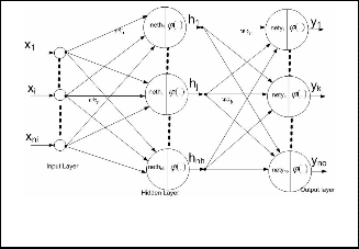

w h ( new ) = w h

(old ) + . k

(14)

k ji

E y

bh (new) = bh (old ) + k

(15)

y bh

E y

wo (new) = wo

(old ) + k

k kj

(16)

E y

bo (new) = bo (old ) + k

(17)

Fig. 5: Architecture of the MLP network

y bk

If the weight that connects the

ith

neuron of the input
where, is the learning rate and
layer with the

j th

neuron of the hidden layer is

w and no k

bias of the

j th

neuron of the hidden layer is bh the net

= [ (1

y ) y w ] (1

h ) h x

(18)

value of the

j th neuron can be given as:

ji k =1

y no

ne t h j =

i =1

( w h ji x i + bh j )

j = 1, 2 , ......., nh

(10)

= [ (1

k =1

y ) y w ] (1

h ) h

(19)

The output of the
j th neutron hj of the hidden layer after

k = (1

y ) y

( 20)

applying activation can be given as bo

1 k

h = < (neth ) =

(11)

= (1

y ) y h

(21)

j j neth

k k j

Similarly the net value “netyk “and the final output yk of kth

International Journal of Scientific & Engineering Research Volume 2, Issue 5, May-2011 5

ISSN 2229-5518

1 N no

( q q )2

(33)

E t y

For different error criterion only

E / y will change and

2 n =1 k =1

is shown as follows: This is dependent on the distance metric used in computation of the total error E.

Then =

(t q

y q )

q y q

(34)

Case 1: Least Mean Square Error

1 N no

LMSE= E = (t y )2

(23)

k k k

k k n =1 k =1

Where, yt denotes the desired vlue of neuron.and ti notes
the target value for the ith pattern.

Then, =

(t y )

k k

(24)

3 Results

Case 2: Geometric error metric
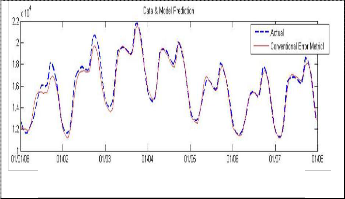
The data is taken from England ISO, and the simulation is

1 N no

E =

[log(

k )]2

(25)

done using MATLAB.the network designed is of two lag- ers with 20 neuron .For converentional model mean abso-

2 n =1

k =1 t

lutes error (MAE) is used. To display the result clearly only forcasting of one week is given. The results are shown in following figures. The x axis in all the figures

Then =

(log(t ) log( y ))

(26)

k k

y y

k k

Case 3: Harmonic error metric
below represents the days (data here shown is only for 1
week; 1st January 2008 to 8th January 2008) and the y axis depict the forecasted load demand (in MW).

E =

N no

( k 1)2

(27)

2 n =1 k =1

Then =

t ( y / t 1)

(28)

k k k

Case 4: Generalized geometric error metric

1 N no

E =

[t r

log( k )]2

(29)

Fig. 6: Forecasting using MAE (conventional model).

2 n =1 k =1

Then =

t r (log(t ) log( y ))

t r

(30)

k k k k

k k

Case 5: Generalized harmonic error metric Type I

1 N no

E = p

( k

1)2

(31)

2 n =1 k =1

Then =

(t p ) ( y / t 1)

(32)

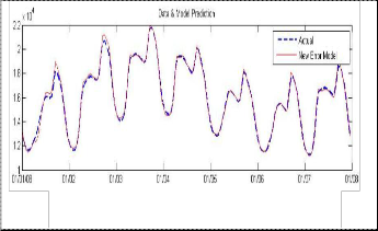
Fig. 7: Forecasting using Generalized Harmonic

k k k

Type I Error Metric

Case 6: Generalized harmonic error metric Type II

International Journal of Scientific & Engineering Research Volume 2, Issue 5, May-2011 6

ISSN 2229-5518

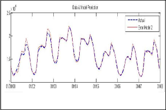
Fig. 8: Forecasting using Generalized Harmonic

Type II Error Metric

learningalgorithmfor radial basis function networks,” IEEE Transactions on Neural Networks, vol. 2, pp.302-309, 1991.

[7] Satish Kumar. : Neural Networks: A Classroom Approach, Tata

McGraw Hill Publishing Company, New Delhi, 3rd Ed. 2007.

[8] W. Schiffmann, M. Joost, and R. Werner, , “Optimization of the backpropagation algorithm for multilayer perceptrons”, Univ. Koblenz, Inst. Physics, Rheinau 3-4, Germany.

[9] R. Battiti, “First and second-order methods for learning:

between steepest descent and Newton’s method”, Neural

Computation, Vol. 2, 141-166, 1992.

[10] J. Yu, J. Amores, N. Sebe, Q. Tian, “Toward an improve Error metric”, International Conference on Image Processing (ICIP), 2004.

[11] J. Yu, J. Amores, N. Sebe, Q. Tian, “Toward Robust Distance Metric Analysis for Similarity Estimation”, IEEE Computer Sosciety Conference on Computer Vision and Pattern Recognition,

2006.

[12] W. J. J. Rey, “Introduction to Robust and Quasi-Robust

Statistical Methods”, Springer-Verlag, Berlin, 110–116, 1983.

[13] K. Hornik, M. Stinchombe and H. White, “Multilayer feedforward networks are universal approximators”, Neural networks, vol. 2, pp. 359-366, 1989.

[14] J. M. Zurada, “Introduction to Artificial Neural Systems”, Jaicob publishing house, India, 2002

[15] G. Cybenko, “Approximation by superpositions of a sigmoidal

function”, Mathematics of Control, Signals, and Systemsvol. 2 pp.303-314, 1989.

Fig. 9: Forecasting using Generalized Geometric

Error Metric

4 CONCLUSION

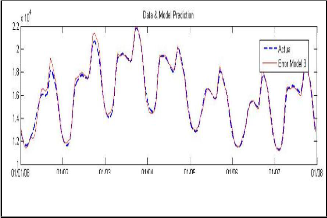
As it is clearly analyazed from the result. The new models are giving better result from the convestional model.this result are justified from the theory that the generalized mean models will capture the variation well.the reason is clear that the variation are largely nonlinear & stocasting in nature so conventional linear models are unable to catch it.

References.

[1] S. Haykin. : Neural Networks: A Comprehensive Foundation,

Macmillan College Publishing Company, New York, 1994

[2] Engle,R.F.,Mustafa,C.,andRice,J. 1992.”Modelling peak electricity Demand”.Journal of forecasting.11:241-251. & Eugene, A.F and Dora,G.2004.Load Forecasting.269-285.State University of New York :New York

[3] D.E. Rumelhart, "Parallel Distributed Processing", Plenary

Lecture presented at Proc. IEEE International Conference on

Neural Networks, San Diego, California, 1988.

[4] Donald F. Specht, “Probabilistic neural networks”, in Neural

Networks, 3, pp. 109-118, 1990

[5] Donald F. Specht, “A General Regression Neural Network”,

IEEE Trans on Neural Networks,Vol 2, 1991.

[6] S. Chen, C.F.N. Cowan, P.M. Grant, “Orthogonal least squares