International Journal of Scientific & Engineering Research, Volume 3, Issue 9, September-2012

ISSN 2229-5518

Improving Sound Quality by Bandwidth

Extension

M. Pradeepa, M.Tech, Assistant Professor

Abstract - In recent telecommunications system uses a limited audio signal bandwidth of 300 to 3400 Hz. In recent times it has been proposed that the mobile phone networks with increased audio signal bandwidth of 50Hz-7 KHz will increase the sound quality of the speech signal. In this paper, a method extending the conventional narrow frequency band speech signals into a wideband speech signals for improved sound quality is proposed. A possible way to achieve an extension is to use an improved speech coder/decoder (CODEC) such as the Adaptive Multi Rate – Wide Band (AMR-WB). However, using an AMR-WB CODEC requires that both telephones at the ends of the communication link support it. Moreover the Mobile phones communicating with wire-line phone can therefore not utilize the enhanced feature of new CODECS; to overcome this limitation the received speech signal can be modified. The modification is meant to artificially increase the bandwidth of the speech signal. The proposed speech bandwidth extension method is Feature Mapped Speech Bandwidth Extension. This method maps each speech feature of the narrow–band signal to a similar feature of the high-band and low- band, which generates the wide band speech signal Y(n).

Index Term - Speech analysis, speech enhancement, speech synthesis

—————————— • ——————————

1 INTRODUCTION

HE far most common way to receive speech signals is di- rectly face to face with only the ear setting a lower fre- quency limit around 20Hz and an upper frequency limit around 20 kHz. The common telephone narrowband speech signal bandwidth of 0.3-3.4 kHz is considerably narrower than what one would experience in a face to face encounter with a sound source, but it is sufficient to facilitate the reliable com- munication of speech. However, there would be a benefit to be obtained by extending this narrowband speech signal to a wider bandwidth in that the perceived naturalness of the
speech signal would be increased.
Speech bandwidth extension (SBE) methods denote tech-
niques for generating frequency bands that are not present in the input speech signal. A speech bandwidth extension meth- od uses the received speech signal and a model for extending the frequency bandwidth. The model can include knowledge of how speech is produced and how speech is perceived by the human hearing system.
Speech bandwidth extension methods have been suggested for a frequency band both at frequencies higher and lower compared with the original narrow frequency band. For con- venience these frequency bands are henceforth termed low- band, narrow-band and high-band. Typical bandwidths used in SBE are 50 Hz–300 Hz, 300 Hz–3.4 kHz, and 3.4 kHz–7 kHz, for the low-band, narrow-band, and high-band, respectively. Ear- ly speech bandwidth extension methods date back more than

————————————————

Pradeepa. M, Assistant Professor, VRS College of Engineering and Tech- nology, Villupuram, Tamilnadu, India, PH- +91 9894694677, E-mail: prathimohan@gmail.com (This information is optional; change it according to your need.)

a decade. Similar to speech CODERs, SBE methods often use an excitation signal and a filter. A simple method to extend the speech signal into the higher frequencies is to up-sample by two neglecting the anti aliasing filter. The lack of antialiasing filter will cause the original spectrum to be mirrored at half the new bandwidth. The wide-band extended signal will have mirrored speech content up to at least 7 kHz. A drawback with this method is the speech-energy gap in the 3.4–4.6 kHz region. The speech-energy gap is the result of telephone bandwidth signals not having much energy above 3.4 kHz. When the speech spectrum is mirrored the speech content in the high-band generally becomes non harmonic even when the narrow-band contains a harmonic spectrum. This is a ma- jor disadvantage of the simple mirroring method.

2 FEATURE MAPPED SPEECH BANDWIDTH EXTENSION

Feature mapped speech bandwidth extension method maps each speech feature of the narrow-band signal to a similar fea- ture of the high-band and low-band. The method is thus named feature mapped speech bandwidth extension (FM- SBE).
A high band synthesis model based on speech signal features
is used. The relation between the narrow-band features and
the high band model is partly obtained from statistical charac- teristics of speech data containing the original high-band. The remaining part of the mapping is based on speech acoustics. The low-complexity of the FM-SBE method is referring to the computational complexity of the mapping from the narrow- band parameters to the wide-band parameters. The FM-SBE method exploits the spectral peaks for estimating the narrow- band spectral vector, neglecting low energy regions in the nar- row-band spectrum.
The FM-SBE method derives an amplitude level of the high band spectrum from logarithm amplitude peaks in the nar- rowband spectrum. FM-SBE method has potential to give a

International Journal of Scientific & Engineering Research Volume 3, Issue 9, September-2012

ISSN 2229-5518

preferred bandwidth extended signal, although the subjects find the amount of introduced distortion too high for all the tested speech bandwidth extension methods, but the system complexity is very low
This paper uses the Feature mapped speech bandwidth exten-
sion method, because its system complexity is low when com-
pared codebook method statistical mapping method , gaussi- an mixture model method(GMM).The proposed speech bandwidth extension method maps each speech feature of the narrow-band signal to a similar feature of the high-band and low-band. The method is thus named feature mapped speech bandwidth extension (FM-SBE).
The feature mapped speech bandwidth extension method is
divided into an analysis and a synthesis part as shown in fig
2.1. The analysis part has the narrow-band signal as input and
results in the parameters that control the synthesis. The syn- thesis will generate the extended bandwidth speech signal. The analysis and synthesis is processed on segments of the input signal. Each segment has a duration of 20ms. The low- band speech synthesized signal, ylow(n;m), and high band speech synthesized signal, yhigh(n;m) , are added to the up- sampled narrow-band signal, ynarrow(n;m) which generates the wide-band speech signal.

y(n;m) = ylow(n;m)+yhigh(n;m)+ynarrow(n;m)
Fig. 2.1 Block Diagram of FM-SBE

3 NARROW BAND SIGNAL ANALYSIS

The analysis part comprises a narrow band speech analyzer, which takes the common narrow band signal as its input and generates the parameter that control the synthesis part. The fig
3.1 shows the narrow band speech signal analysis part.

Fig 3.1 Narrow band speech signal analysis

The block diagram shows the narrow band speech signal analysis of the Feature mapped speech bandwidth extension (FM-SBE) method. The narrow band speech signal analysis part consists of linear predictor, AR spectrum and Pitch fre- quency determination blocks. The narrow band analysis takes speech signal as input signal. This speech signal is divided into number of short time segment of duration 20ms. The analysis is carried out for each short time segment. The short duration signal is applied to the linear prediction. The term
‘linear prediction’ refers to the prediction of the output of a linear system based on its input sequence. The linear predic-
tion gives the residual signal, filter coefficient and autocorrela- tion. Using the autocorrelation the AR method is used to cal- culate the power spectral density of the signal.
From this, the peaks and frequency corresponding to the
peaks are calculated. The number of peaks in an AR spectrum is approximately half the number of filter co-efficient. The pitch frequency is also estimated for each segment. The indi- vidual blocks are dealt in detail in the following section.

4 LOW-BAND SPEECH SIGNAL SYNTHESIS

Fig 4.1 Block diagram of low-band speech signal synthesis
The Fig 4.1 shows the block diagram of low-band speech sig- nal synthesis. It consists of gain, continuous sine tones genera- tor and low pass filter blocks. The narrow bandwidth tele- phone speech signal has a lower cutoff frequency of 300 Hz. On a perceptual frequency scale, such as the Bark-scale, the low-band covers approximately three Bark-bands and the high-band covers four Bark-bands. This gives that the low- band is almost as wide as the high-band on a perceptual scale. During voiced speech segments most of the speech content in the low-band consists of the pitch and harmonics. During un- voiced speech segments the low-band is not perceptually im- portant.
The suggested method of synthesizing speech content in the low-band is to introduce sine tones at the pitch frequency ω and the harmonics up to 300 Hz. Generally, the number of tones is five or less since the pitch frequency is above 50 Hz.

International Journal of Scientific & Engineering Research Volume 3, Issue 9, September-2012

ISSN 2229-5518

This is done by the continuous sine tone generator and LPF
blocks.
The harmonics generated by the glottal source are shaped by the resonances in the vocal tract. In the low-band the lowest resonance frequency is important. The first formant is in the approximate range of 250–850 Hz during voiced speech. This gives that, the natural amplitude levels at the harmonics in the frequency range 50–300 Hz are either approximately equal or have a descending slope toward lower frequencies. Low fre- quency tones can substantially mask higher frequencies when a high amplitude level is used. Masking denotes the phenom- ena when one sound, the masker, makes another sound, the masked, in-audible. The risk of masking gives that caution must be taken when introducing tones in the low-band. The amplitude level of all the sine tones is adaptively updated with a fraction of the amplitude level of the first formant by the gain adjustment block where the gain g1(m) is given by
g1(m) = C1 . P(1:m) (1)
where C1 is a constant fraction substantially less than one to ensure only limited masking will occur. Therefore the low band signal Ylow(n) are the continuous sine tone frequencies at the pitch frequency and its harmonics.

5 HIGH-BAND SPEECH SIGNAL SYNTHESIS

The high-band speech synthesis generates a high-frequency spectrum by shaping an extended excitation spectrum. The excitation signal, , is extended up-wards in frequency. A simple method to accomplish this is to copy the spectrum from lower frequencies to higher frequencies.
The method is simple since it can be applied in the same manner on any excitation spectrum. During the extension it is essential to continue a harmonic structure.
Most of the higher harmonics cannot be resolved by the hu- man hearing system. However, a large enough deviation from a harmonic structure in the high-band signal could lead to a rougher sound quality.

Previously a pitch-synchronous transposing of the excitation spectrum has been proposed which continues a harmonic spectrum. This transposing does not take into consideration the low energy level at low frequencies of telephone band- width filter signals, giving small energy gaps in the extended spectrum. Energy gaps are avoided with the present method since the frequency-band utilized in the copying is within the narrow-band. The full complex excitation spec- trum, , is calculated on a grid, i= 0,……., I-1 , of fre-
quencies using an FFT of the excitation signal The
spectrum of the excitation signal is divided into zones: the
lower match zone and the higher match zone. The Fig 5.1 shows the block diagram of high band speech signal synthesis. The prediction error is the input of the high band speech sig- nal synthesis. After taking FFT, the spectrum of the excitation signal is divided into two zones ie., lower match zone and higher match zone. The frequency range of lower match zone is 300Hz and higher match is 3400Hz. The spectrum between two zones ie., 300Hz to 3400Hz is copied repeatedly to the

range from 3400Hz to 7000Hz. After taking IFFT the high band speech signals are generated.
Fig 5.1 Block diagram of high-band speech signal synthesis

6 SPEECH QUALITY EVALUATION

Synthetic speech can be compared and evaluated with respect to intelligibility, naturalness, and suitability for used applica- tion. In some applications, for example reading machines for the blind, the speech intelligibility with high speech rate is usually more important feature than the naturalness. On the other hand, prosodic features and naturalness are essential when we are dealing with multimedia applications or elec- tronic mail readers.
The evaluation can also be made at several levels, such as
phoneme, word or sentence level, depending what kind of
information is needed. Speech quality is a multi-dimensional term and its evaluation contains several problems. The evalua- tion methods are usually designed to test speech quality in general, but most of them are suitable also for synthetic speech. It is very difficult, almost impossible, to say which test method provides the correct data. In a text-to-speech system not only the acoustic characteristics are important, but also text pre-processing and linguistic realization determine the final speech quality. Separate methods usually test different properties, so for good results more than one method should be used. And finally, how to assess the test methods them- selves.The evaluation procedure is usually done by subjective listening tests with response set of syllables, words, sentences, or with other questions. The test material is usually focused on consonants, because they are more problematic to synthesize than vowels. Especially nasalized consonants (/m/ /n/ /ng/) are usually considered the most problematic. When using low bandwidth, such as telephone transmission, consonants with high frequency components (/f/ /th/ /s/) may sound very annoying. Some consonants (/d/ /g/ /k/) and consonant combinations (/dr/ /gl/ /gr/ /pr/ /spl/) are highly intelli- gible with natural speech, but very problematic with synthe- sized one. Especially final /k/ is found difficult to perceive. The other problematic combinations are for example /lb/,
/rp/, /rt/, /rch/, and /rm/. Some objective methods, such as
Articulation index (AI) or Speech Transmission Index (STI), have been developed to evaluate speech quality. These meth- ods may be used when the synthesized speech is used through

International Journal of Scientific & Engineering Research Volume 3, Issue 9, September-2012

ISSN 2229-5518

some transmission channel, but they are not suitable for eval- uating speech synthesis in general. This is because there is no unique or best reference and with a TTS system, not only the acoustic characteristics are important, but also the implemen- tation of a high-level part determines the final quality. How- ever, some efforts have been made to evaluate objectively the quality of automatic segmentation methods in concatenative synthesis.
They are two possible way to measure the sound quality

• Subjective speech quality measures.

• Objective speech quality measures.

6.1 Subjective Speech Quality Measures

Speech quality measures based on ratings by human listeners are called subjective speech quality measures.
These measures play an important role in the development of
objective speech quality measures because the performance of objective speech quality measures is generally evaluated by their ability to predict some subjective quality assessment. Human listeners listen to speech and rate the speech quality according to the categories defined in a subjective test.
The procedure is simple but it usually requires a great amount of time and cost. These subjective quality measures are based on the assumption that most listeners’ auditory responses are similar so that a reasonable number of listener scan represent all human listeners. To perform a subjective quality test, hu- man subjects (listeners) must be recruited, and speech samples must be determined depending on the purpose of the experi- ments. After collecting the responses from the subjects, statis- tical analysis is performed for the final results.
Two subjective speech quality measures used frequently to
estimate performance for telecommunication systems are

• Mean Opinion Score

• Degradation Mean Opinion Score

6.2 Mean Opinion Score (MOS)

MOS is the most widely used method in the speech coding community to estimate speech quality. This method uses an absolute category rating (ACR) procedure. Subjects (listeners) are asked to rate the overall quality of a speech utterance be- ing tested without being able to listen to the original reference, using the following five categories as shown in Table 6.1. The MOS score of a speech sample is simply the mean of the scores collected from listeners.

TABLE 6.1

MOS and Corresponding Speech Quality

An advantage of the MOS test is that listeners are free to as-
sign their own perceptual impression to the speech quality. At the same time, this freedom poses a serious disadvantage be- cause individual listeners’ “goodness” scales may vary greatly [Voiers, 1976]. This variation can result in a bias in a listener’s judgments. This bias could be avoided by using a large num- ber of listeners. So, at least 40 subjects are recommended in order to obtain reliable MOS scores [ITUT Recommendation P.800, 1996].

6.3 Degradation Mean Opinion Score (DMOS)

In the DMOS, listeners are asked to rate annoyance or deg- radation level by comparing the speech utterance being tested to the original (reference). So, it is classified as the degradation category rating (DCR) method. The DMOS provides greater sensitivity than the MOS, in evaluating speech quality, be- cause the reference speech is provided. Since the degradation level may depend on the amount of distortion as well as dis- tortion type, it would be difficult to compare different types of distortions in the DMOS test. Table 6.2 describes the five DMOS scores and their corresponding degradation levels.

TABLE 6.2

MOS and Corresponding Speech Quality

Thorpe and Shelton (1993) compared the MOS with the DMOS in estimating the performance of eight codecs with dynamic background noise [Thorpe and Shelton, 1993]. According to their results, the DMOS technique can be a good choice where the MOS scores show a floor (or ceiling) effect compressing the range. However, the DMOS scores may not provide an estimate of the absolute acceptability of the voice quality for the user.

6.4 Objective Speech Quality Measures

An ideal objective speech quality measure would be able to assess the quality of distorted or degraded speech by simply observing a small portion of the speech in question, with no access to the original speech [Quackenbush et al., 1988]. One attempt to implement such an objective speech quality meas- ure was the output-based quality (OBQ) measure [Jin and Kubicheck, 1996]. To arrive at an estimate of the distortion using the output speech alone, the OBQ needs to construct an internal reference database capable of covering a wide range of human speech variations. It is a particularly challenging problem to construct such a complete reference database. The performance of OBQ was unreliable both for vocoders and for various adverse conditions such as channel noise and Gaussi- an noise.

International Journal of Scientific & Engineering Research Volume 3, Issue 9, September-2012

ISSN 2229-5518

Current objective speech quality measures base their esti- mates on both the original and the distorted speech even though the primary goal of these measures is to estimate MOS test scores where the original speech is not provided.
Although there are various types of objective speech quali-
ty measures, they all share a basic structure composed of two

components as shown in fig 6.1.
Fig. 6.1 Objective Speech Quality Measure Based on Both Orig- inal and reconstructed Speech
The original speech signal is applied for speech bandwidth extension and it produces the reconstructed speech signal. Then the original speech signal and reconstructed speech sig- nal are compared for objective speech quality measure. In this project, the objective speech quality is measured by the time domain measure signal-to-noise ratio (SNR).

7 STIMULATION RESULTS

7.1 Speech signal without noise

For the experimental setup, the proposed method utilized

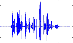
The speech signal of length 3sec is taken from the TIMIT database and this speech signal is divided into number of segments, each of 20msec as shown in fig 7.1.2. The fig 7.1.3 shows the up-sampled speech signal segment. The up- sampled signal is refers as increasing the sampling frequency rate by 2. A sample of each segment and the parameters esti- mated for each segment are shown.

Fig 7.1.2 Speech signal segments

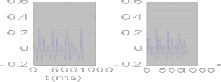
Fig. 7.1.3 Up-sampled Speech signal segments
LP analysis
To avoid the interaction of harmonics and noise signals, the
proposed method operates on the linear prediction residual signal. The residual signal is also called as prediction error. The Fig 7.1.4 shows the estimated signal from LP for speech signal segment and fig 7.1.5 shows the residual signal after LP for speech signal segment.
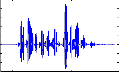
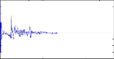
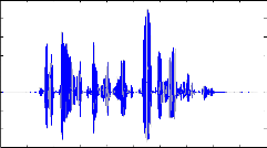
speech signals from TIMIT database (so called because the data were collected at Texas instrument (TI) and annotated at Massachusetts Institute of Technology (MIT)), which are sam- pled at 16 KHz. The Fig 7.1.1 shows the speech waveform of speech ‘CHEMICAL EQUIPMENT NEED PROPER MAINTANENCE’.

Speech signal

0.6

0.4

0.2

- 0.2

0 200 400 t (ms)

0.6

0.4

0.2

- 0.2

0 200 400

0.5

0.4

0.3

0.2

0.1

-0.1

-0.2

-0.3

0 0.5 1 1.5 2 2.5 3 3.5 4 4.5 5

Fig 7.1.4 Estimated signal from LP

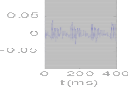
Fig 7.1.5 Residual signal after LP

Time in ms

Fig 7.1.1 Speech signal waveform

Segmentation

x 10

International Journal of Scientific & Engineering Research Volume 3, Issue 9, September-2012

ISSN 2229-5518

Autocorrelation
The Figure 7.1.6 shows the autocorrelation of the linear predic- tion. The autocorrelation refers to the similarities between the two same signals.

0.015

0.01

0.005

- 0.005

- 0.01

- 0.015

0 0.01 0.02 0.03 0.04 0.05 0.06 0.07 0.08 t (ms)

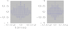
Fig 7.2.2 Unvoiced segment

Fig 7.1.6 Autocorrelation
Pitch frequency

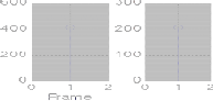
The Fig 7.1.7 shows the pitch frequency of the speech signal. Pitch frequency is determined for each segment. Pitch fre- quency is also called as fundamental frequency of the vocal cord. Pitch frequency is the difference between the two peak amplitudes. This figure shows the pitch frequency for each speech signal segment.

Fig 7.1.7 Pitch frequency

7.2 Low band speech signal

The fig 7.2.1 and 7.2.2 show the sine wave of low band speech signal for voiced and unvoiced segments. The sine waves are generated by using the pitch frequency and first peak power. For voiced segment, harmonics will occur but in the case of unvoiced segment no harmonics will occur because the fre- quency range of voiced segment is 150Hz and the frequency range of unvoiced segment is 400Hz. The low band frequency range is 50Hz to 300Hz.

0.03

0.02

0.01

- 0.01

- 0.02

- 0.03

0 0.01 0.02 0.03 0.04 0.05 0.06 0.07 0.08

t (ms)

Fig 7.2.1 Voiced segment
Added signal of up-sampled signal and low band speech signal
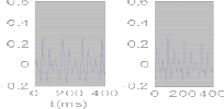
The Fig 7.2.3 and 7.2.4 show the addition of up-sampled speech signal segment and low band speech signal segment for voiced and unvoiced segments.

Fig 7.2.3 Voiced segment

Fig 7.2.4 Unvoiced segment

7.3 High band speech signal

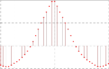
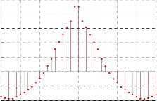
The Fig 7.3.1 and 7.3.4 show the FFT of the prediction error for voiced segment and unvoiced segment. After taking FFT, the spectrum of the excitation signal is divided into two zones ie., lower match zone and higher match zone. The frequency range of lower match zone is 300Hz and higher match is
3400Hz. The spectrum between two zone 300Hz to 3400Hz is copied repeatedly to the range from 3400Hz to 7000Hz.The Fig
7.3.2 and 7.3.5 show the spectral copy of the FFT of the predic- tion error for voiced segment and unvoiced segment. The Fig
7.3.3 and 7.3.6 show the IFFT of the spectral copy for voiced
and unvoiced segment.

International Journal of Scientific & Engineering Research Volume 3, Issue 9, September-2012

ISSN 2229-5518

0.8

0.6

0.4

- 3

x 10

0.2

- 0.2

- 0.4

- 0.6

0 500 1000 1500 2000 2500 3000 3500 freq in Hz

- 1

- 2

0 1000 2000 3000 4000 5000 6000 7000

freq in Hz

Fig 7.3.1 FFT of prediction error for voiced segment

Fig 7.3.5 Spectral copy of the FFT of prediction error for unvoiced seg- ment

0.8

- 3

x 10

0.6 6

0.4

0.2 0

- 2

- 4

- 0.2 - 6

- 0.4

- 8

0 100 200 300 400 500 600 700 800

Time in ms

- 0.6

0 1000 2000 3000 4000 5000 6000 7000 freq in Hz

Fig 7.3.6 IFFT of the spectral copy for unvoiced segment

Fig 7.3.2 Spectral copy of the FFT of prediction for voiced segment

0.25

0.2

0.15

0.1

0.05

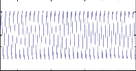
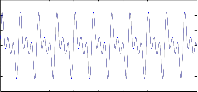
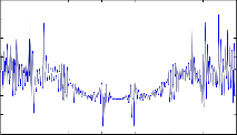
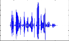
7.4 Wide band speech signal

The Figure 7.4.1 shows the wide band speech signal after the FM-SBE method. The synthesis part generates upper band and lower band speech signal. These upper band and lower band speech signal are added to up-sampled narrow band speech signal to generate the wide band speech signal of improved quality.

0.5

0.4

0.3

- 0.05

- 0.1

0 100 200 300 400 500 600 700 800 t ime in ms

0.2

0.1

Fig 7.3.3 IFFT of the spectral copy for voiced segment

- 0.1

- 0.2

- 0.3

- 3

0 2 4 6 8 10

x 10

Time in ms

Fig 7.4.1 Wide band speech signal
Objective sound quality measure

x 10

- 1

- 2

0 500 1000 1500 2000 2500 3000 3500

freq in Hz

Fig 7.3.4 FFT of prediction error for unvoiced segment
For objective sound quality measure two ways to measure the
sound quality are carried out. One is SNR measurement and the other is cross correlation measurement. The Table 7.1 shows the SNR measurement for original and reconstructed
speech signal, the SNR of 35db and 50db noisy speech and its reconstructed noisy speech signal.

International Journal of Scientific & Engineering Research Volume 3, Issue 9, September-2012

ISSN 2229-5518

Table 7.1
SNR measurement

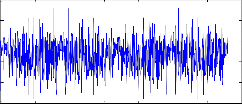
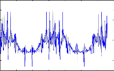
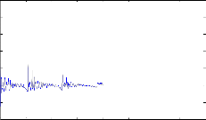
The figures 7.4.2 and 7.4.3 show the original speech signal and reconstructed speech signal. The figure 7.4.4 shows the cross correlation between original and reconstructed speech signal and its peak value is 1.
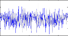
Fig 7.4.5 Speech signal with AWGN noise

0.5

0.4

0.3

0.2

0.1

-0.1

-0.2

-0.3

Speech signal

0 0.5 1 1.5 2 2.5 3 3.5 4 4.5 5

Time in ms

Fig 7.4.2 Original speech signal

x 10

0.5

Sample Cross Correlat ion Funct ion (XCF)

Fig 7.4.6 Reconstructed noisy speech signal
The fig 7.4.5 and 7.4.6 show the noisy speech signal and recostructed noisy speech signal. The fig 7.4.7 shows the cross correlation between noisy speech signal and reconstructed noisy speech signal.

- 0.5

- 20 - 15 - 10 - 5 0 5 10 15 20

Lag

Fig 7.4.3 Reconstructed speech signal

0.5

0.4

0.3

0.2

0.1

0.8

0.6

0.4

0.2

- 0.2

Sample Cross Correlat ion Funct ion (XCF)

- 0.1

- 0.2

- 0.3

0 2 4 6 8 10

- 0.4

- 20 - 15 - 10 - 5 0 5 10 15 20

Lag

Time in ms

x 10

Fig 7.4.7 Cross correlation of original and reconstructed noisy
Fig 7.4.4 Cross correlation of original and reconstructed speech
signal
speech signal

International Journal of Scientific & Engineering Research Volume 3, Issue 9, September-2012

ISSN 2229-5518

8 CONCLUSION AND FUTURE WORK

Telecommunication uses a limited audio signal bandwidth of 0.3-
3.4 kHz, but it will affect the sound quality when compared to face to face communication. So extending the bandwidth from narrow band to wide band in mobile phone is suggested. A pos- sible way to achieve an extension is to use an improved speech COder/DECoder (CODEC) such as the adaptive multi rate wide band. But this method has some drawbacks. Many speech band- width extension methods such as codebook method, statistical mapping method, guassian mixture model and feature mapped speech bandwidth extension method can provide better system performance. These methods are used to extend the narrow band speech signal to wide band speech signal. But these methods (codebook, statistical, GMM) require more computation. This project employs a FM-SBE method which provide low complexi- ty and improves the sound quality of the speech signal at the re- ceiver side.
The proposed method consists of analysis part and synthesis part.
From analysis part the speech parameters are estimated. It is ob- served that the prediction error is more in unvoiced and silent segment when compared to voiced because the linear predictor has been designed with the filter coefficient such that it estimate voice with less error. This is because we are more interested in predicting the voice better than the unvoiced and silent. In the synthesis part, the upper band speech synthesis and lower band speech synthesis are generated. The upper band speech synthesis and lower band speech synthesis are added to the up-sampled narrow band speech signal, which generates the wide band speech signal. By employing FM-SBE method wide band speech signal with enhanced quality is obtained. Speech quality has been tested by objective measure such as SNR and autocorrelation and results indicate that speech quality is good. A different level of noise was added to the speech signal and quality of the recon- structed speech with and without noise was tested objectively and subjectively.
In the current work, narrow band speech signal is first analyzed
and parameters are extracted. To improve speech quality, a lower band and a upper band are synthesized and added to the narrow band speech. Future work can focus on improvement of the speech quality by using fricated speech quality detector. The fricated speech gain is used to detect when the current speech segment contains fricative or affricate consonants. This can then be used to select a proper gain calculation method. Similarly im- provement can be done by adding a voice activity detector, which can detect when bandwidth extension has to be carried out.

REFERENCES

[1] “DARPA-TIMIT”Acoustic-Phonetic Continuou Speech Corpus, NIST Speech Disc 1-1.1, 1990.

[2] H.Gustafsson, U.A.Lindgren and I.Claesson,” Low-Complexity Fea-

ture-Mapped Speech Band width Extension”, IEEE Transaction on Au- dio, Speech and Language Processing vol.14, no.2, pp.577-588, March

2006.

[3] J. Epps and H. Holmes, “A new technique for wide- band enhance- ment of coded narrow-band speech”, Proceedings of IEEE Workshop on Speech Coding, pp. 174–176, April 1999

[4] M. Nilsson, H. Gustafsson, S. V. Andersen, and W.B.Kleijn, “Gauss-

ian mixture model and mutual information estimation between fre- quency bands in speech”,Proceeding of International Conference on Acoustics, Speech, Signal Processing, Swedan, vol.10, no. 23, July 2002.

[5] M.Budagavi and J.D.Gibson,”Speech Coding in Mobile Radio Com-

munications”, Proceedings of the IEEE, vol.86, no.8, pp. 1402-1412, July,

1998.

[6] S.Spanias, “Speech coding: a tutorial review”, Proceedings of the IEEE, vol.82, no.2 pp.1541-1582, Oct. 1994.

[7] Technical Specification Group Services and System Aspects; Speech Codec Speech Processing Functions; AMR Wide-band Speech Codec; Transcoding Functions, TS 26.190 v5.1.0, 2001.

[8] W. Hess, Pitch Determination of Speech Signals. New York: Springer-

Verlag, 1983.

[9] William M. Fisher, George R. Doodington, and Kathleen M. Goudie- Marshall, “The DARPE Speech Recognition Research Database: Specifications and Status”, Proceedings of DARPA Workshop on Speech recognition, pp. 93-99, February 1986.

[10] Y. M. Cheng, D. O’Shaughnessy, and P. Mermelstein, “Statistical re-

covery of wide-ban Speech from narrow-band speech”, Proceedings of International Conference on Speech and Language Processing, Edinburgh, vol.17, no.3, pp.1577-1580, September 1992.