International Journal of Scientific & Engineering Research, Volume 4, Issue 8, August-2013 1216

ISSN 2229-5518

Improved Short Term Wind Power Prediction

Using A Combined Locally Weighted GMDH

and KPCA

E. E. Elattar, Member, IEEE, I. Taha and Kamel A. Shoush

Abstract— W ind power prediction is one of the most critical aspects in wind power integration and operation. This paper proposes a new approach for wind power prediction. The proposed method is derived by integrating the kernel principal component analysis (KPCA) method with the locally weighted group method of data handling (LWGMDH) which can be derived by combining the GMDH with the local regression method and weighted least squares (W LS) regression. In the proposed model, KPCA is used to extract features of the inputs and obtain kernel principal components for constructing the phase space of the multivariate time series of the inputs. Then LW GMDH is employed to solve the wind power prediction problem. The coefficient parameters are calculated using the W LS regression where each point in the neighborhood is weighted according to its distance from the current prediction point. In addition, to optimize the weighting function bandwidth, the weighted distance algorithm is presented. The proposed model is evaluated using real world dataset. The results show that the proposed method provides a much better prediction performance in comparison with other models employing the same data.

Index Terms— W ind power prediction, group method of data handling, local predictors, locally weighted group method of data handling, weighted distance, kernel principal component analysis, state space reconstruction.

——————————  ——————————

1 INTRODUCTION

IND power is the fastest growing power generation sector in the world nowadays. The output power of wind farms is hard to control due to the uncertain and
variable nature of the wind resources. Hence, the integration of a large share of wind power in an electricity system leads to some important challenges to the stability of power grid and the reliability of electricity supply [1]. Wind power prediction is one of the most critical aspects in wind power integration and operation. It allows scheduled operation of wind turbines and conventional generators, thus achieves low spinning re- serve and optimal operating cost [2].
Short term prediction is generally for a few days, and hours to a few minutes, respectively. It is required in the gen- eration commitment and market operation. Short term wind power prediction is a very important field of research for the energy sector, where the system operators must handle an important amount of fluctuating power from the increasing installed wind power capacity. Its time scales are in the order of some days (for the forecast horizon) and from minutes to hours (for the time-step) [3].
Various methods have been identified for short term wind
power prediction. They can be categorized into physical
methods, statistical methods, methods based upon artificial

————————————————

• This work was supported byTaif University, KSA under grant 2742-434-1.

• The Authors are with the department of the Electrical Engineering, Faculty of Engineering, Taif University, KSA.

• E. E. Elattar on leave from the Department of Electrical Engineering, Faculty of Engineering, Menofia University, Shebin El-Kom, Egypt

(e-mail: dr.elattar10@yahoo.com).

• I. Taha is on leave from the Department of Electrical Power and Machines,

Faculty of Engineering, Tanta University, Tanta, Egypt.

• Kamel A. Shoush is on leave from the Department of Electrical Engineer- ing, Faculty of Engineering, Al-Azhar University, Cairo, Egypt.
intelligence (AI) and hybrid approaches [4].
The physical method needs a lot of physical considera-
tions to give a good prediction precision. It is usually used for long term prediction [5]. While the statistical performs well in short term prediction [6].
The traditional statistical methods are time-series-based methods, such as the persistence method [7], auto regressive integrated moving average (ARIMA) method [8], [9], etc. These methods are based on a linear regression model and can not always represent the nonlinear characteristics of the in- puts. The AI methods describe the relation between input and output data from time series of the past by a non-statistical approach such as artificial neural network (ANN) [10], [11], fuzzy logic [7] and neuro-fuzzy [12]. Moreover, other hybrid methods [13], [14] have also been applied to short-term wind power prediction with success.
Support vector regression (SVR) [15] has been applied to wind speed prediction with success [16]. SVR has been shown to be very resistant to the overfitting problem and gives a high generalization performance in prediction problems. SVR has been evaluated on several time series datasets [17].
The Group Method of Data Handling (GMDH) is a selfor- ganizing method that was firstly developed by Ivakhnenko [18].The main idea of GMDH is to build an analytical function in a feedforward network based on a quadratic node transfer function whose coefficients are obtained using a regression technique [19]. GMDH has been applied to solve many predic- tion problems with success [20], [21].
All the above techniques are known as global time series predictors in which a predictor is trained using all data availa- ble but give a prediction using a current data window. The global predictors suffer from some drawbacks which are dis- cussed in the previous work [22].

International Journal of Scientific & Engineering Research, Volume 4, Issue 8, August-2013 1217

ISSN 2229-5518

The local SVR method is proposed by us to overcome the drawbacks of the global predictors [22]. More details of the local predictor can be found in [22]. Phase space reconstruc- tion is an important step in local prediction methods. The tra- ditional time series reconstruction techniques usually use the coordinate delay (CD) method [23] to calculate the embedding dimension and the time delay constant of the time series [24].
The traditional time series reconstruction techniques have a serious problem. In which there may be correlation be- tweendifferent features in reconstructed phase space. Conse- quently, the quality of phase space reconstruction and model- ling will be affected [25]. In recent years, to process nonlinear time series, the kernel principal component analysis (KPCA) which is one type of nonlinear principal component analysis (PCA) is used [26]. KPCA is an unsupervised technique that is based on performing principal component analysis in the fea- ture space of a kernel. The main idea of KPCA is first to map the original inputs into a high-dimensional feature space via a kernel map, which makes data structure more linear, and then to calculate principal components in the high-dimensional feature space [25].
Moreover, our previous work on local SVR predictor is ex- tended to locally weighted support vector regression (LWSVR) by modifying the risk function of the SVR algorithm

2 TIME SERIES RECONSTRUCTION BASED ON KPCA

The PCA is a well-known method for feature extraction [29]. It involves the computations in the input (data) space so it is a linear method in nature. KPCA is an unsupervised tech- nique that is based on performing principal component analy- sis in the feature space of a kernel. KPCA can be used to re- construct the time series, on the basis of which some kernel principal components are chosen according to their correlative degree to the model output to form final phase space of the- nonlinear time series.
In KPCA the computations are performed in a feature space that is nonlinearly related to the input space. This fea- ture space is that defined by an inner product kernel in ac- cordance with Mercer’s theorem [30]. Due to the nonlinear relationship between the input space and feature space the KPCA is nonlinear. However, unlike other forms of nonlinear PCA, the implementation of KPCA relies on linear algebra by mapping the original inputs into a high-dimensional feature space via a kernel map, which makes data structure more line- ar.
The basic idea of KPCA is to map the data x into a high
dimensional feature space Φ(𝑥) via a nonlinear mapping,
and perform the linear PCA in that feature space:
with the use of locally weighted regression (LWR) while keep- ing the regularization term in its original form [27], [28].

Q( xi , x j ) = Φ( xi ) ⋅ Φ( x j )

(1)
LWSVR has been applied to solve short term load forecasting
(STLF) problem [27], [28]. Although LWSVR method improves
where xi and xj are variables in input space and 𝑄�𝑥𝑖 , 𝑥𝑗 � is
called kernel function.

𝑁 𝑛

the accuracy of STLF, it suffers from some limitations. First,
the most serious limitation of SVR algorithm is uncertain in choice of a kernel. The best choice of kernel for a given prob- lem is still a research issue. The second limitation is the selec- tion of SVR parameters due to the lacking of the structural
Given a set of data 𝑋 = {𝑥𝑖 }𝑖 =1 where each 𝑥𝑖 ∈ ℜ , we have a corresponding set of feature vector {Φ(𝑥𝑖 )}N . Accordingly, the sample covariance matrix Φ(𝑥𝑖 ) can be de-
fines as follows:
~ N T
methods for confirming the selection of parameters efficiently. Finally, the SVR algorithm is computationally slower than the
C = ∑ Φ( xi )Φ

i =1

( xi )
(2)
artificial neural networks.
To avoid the limitations of the existing methods and in order to follow the latest developments to have a modern sys-
As in PCA method, we have to ensure that the set of feature
vectors {Φ(𝑥𝑖 )}N have zero mean [31]:
1 N
tem, a new method is proposed in this paper using an alterna-
tive machine learning technique which is called GMDH.

∑ Φ( xi ) = 0

i =1

(3)
The proposed method is derived by combining the GMDH with the local regression method and weighted least squares regression and employing the weighted distance algo- rithm which uses the Mahalanobis distance to optimize the weighting function’s bandwidth. In the proposed model, the phase space is reconstructed based on KPCA method, so that the problem of the traditional time series reconstruction tech- niques can be avoided. The proposed method has been evalu- ated using real world dataset.
The paper is organized as follows: Section 2 describes the time series reconstruction based on KPCA method. Section 3 reviews the GMDH algorithm. The LWGMDH method is in- troduced in Section 4. Section 5 describes the weighted dis-
tance algorithm. Experimental results and comparisons with
Proceeding then on the assumption that the feature vectors have been centered, KPCA solves the eigenvalues (4):
𝜆𝑖 𝑣𝑖 = 𝐶̃𝑣𝑖 , i=1,2,….., N (4)
where 𝜆𝑖 is one of the non-zero eigenvalues of 𝐶̃ and 𝑣𝑖 is the
corresponding eigenvectors. Because the eigenvectors 𝑣𝑖 in the
plane which is composed of Φ(𝑥1 ), Φ(𝑥2 ), … . . Φ(𝑥𝑁 ). Therefore
[25]:
𝜆𝑖 𝛷(𝑥𝑖 ) ∙ 𝑣𝑖 = Φ(𝑥𝑖 ) ∙ 𝐶̃𝑣𝑖 , i=1,2,….., N (5)
And the exist coefficient α meet:

other methods are presented in Section 6. Finally, Section 7 concludes the work.

v = ∑α j Φ( x j )

j =1

(6)

International Journal of Scientific & Engineering Research, Volume 4, Issue 8, August-2013 1218

ISSN 2229-5518

Substituting (2) and (6) into (4) and defining an 𝑁 × 𝑁 matrix
Q which is defined by (1), the following formula can be got
[30]:

N N N

∑ ∑α j Φ( xi ) Q ( xi , x j ) = Nλ ∑α j Φ( x j )

(7)

i =1

j =1

Eq. (7) can be written in the compact matrix form [30]:

Nλα = Qα

(8)
Assuming the eigenvectors of

Φ( xi ) is of unit length vi .

vi = 1 , each αi must be normalized using the corresponding eigen-
value by: . ~

α i ,

Nλi

i = 1,2,....., N

Finally the principal component for xi , based on αi , can be
calculated as following:

p (i) = v T Φ( xi ) = ∑α j Φ( xi , x j ),

i = 1,2,..., N

(9)

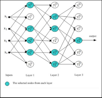
Fig. 1. GMHD network

t i

j =1

From (9), one can notice that the maximal number of prin- cipal components that can be extracted by KPCA is N. The dimensional of pt can be reduced in KPCA by considering the first several eigenvectors that is sorted in descending order of the eigenvalues.
In this paper, we can employ the commonly used Gaussian kernel defined as:
The corresponding network as shown in Fig. 1 can be con- structed from simple polynomial. As the learning procedure evolves, branches that do not contribute significantly to the specific output can be deleted; this allows only the dominant causal relationship to evolve.
The GMDH network training algorithm procedures can be

Q( xi , x)

= exp(−

xi − x )

2σ 2

(10)
summarized as follows:

• GMDH network begins with only input nodes and all

combinations of different pairs of them are generated

3 GROUP METHOD OF DATA HANDLING (GMDH)

Suppose that the original dataset consists of M columns of the values of the system input variables that is X = ( x1 (t), x2 (t),....., x M (t)), (t = 1,2,..., N and a column of the observed values of the output and N is the length of the da- taset.

The connection between inputs and outputs variables can be represented by a finite Volterra-Kolmogorov-Gabor poly- nomial of the form:

using a quadratic polynomial using (Eq. 12) and sent into the first layer of the network. The total number of polynomials (nodes) that can constructed is equal to M(M-1)/2.

• Use list squares regression to compute the optimal

coefficients of each polynomial (node) A(a0 , a1 , a3 , a4 , a5 ) to make it best fit the training data as following:

1 ~ 2

N N N

e = ∑ ( yi − yi )

(13)

y = a

+ ∑ a x + ∑ ∑ a x x
+ ∑ ∑ ∑ a

x x x

+ ...
(11)

i =1

0 i i

i =1

i =1 j =1

ij i j

i =1 j =1 k =1

ijk i j k

The least square solution of (Eq. 13) is given by:

Where N is the number of the data of the dataset, A(a0 , ai , aij ,

aijk, …..) and X(xi , xj , ak ,…..) are vectors of the coefficients and input variables of the resulting multi-input single-output sys-

A = ( X T X ) −1 X T Y

(14)
tem, respectively.
In the GMDH algorithm, the Volterra-Kolmogorov-Gabor
Where, Y = [ y1 , y 2
, ........., y N
]T ,
series is estimated by a cascade of second order polynomials using only pairs of variables [18] in the form of:

1 x1P



x1Q

x1P

x1Q

2 2

1P 1Q

2 2 

~ 2 2

1 x2 P



x1Q

x2 P x2Q

x2 P

x2Q 



y = a0 + a1 xi + a 2 x j + a3 xi x j + a 4 xi

+ a5 x j

(12)

X = . . . .



. . . .

1 x x x x

. .



. . 

x 2 x 2 

 NP

NQ NP NQ

NP QP 

International Journal of Scientific & Engineering Research, Volume 4, Issue 8, August-2013 1219

ISSN 2229-5518

and

P, Q ∈{1, 2,.., M }

• Compute the mean squared error for each node (Eq.
13).
• Sort the nodes in order of increasing error.
• Select the best nodes which give the smallest error
from the candidate set to be used as input into the
where w is the weighting function. Meany weighting func- tions are proposed by the researchers [32]. Out of theses weighting functions, Gaussian kernel, tricube kernel and quadratic kernel are the most popular [32]. In this work, we employ the commonly used Gaussian kernel weighting function as following:
next layer with all combinations of different pairs of them being sent into second layer.
• This process is repeated until the current layer is
found to not be as good as the previous one. There-

wi =

exp(

xi − xq

)

(16)
fore, the previous layer best node is then used as the
where

xq is the query point,

xi is a data point belongs the

final solution.
nearest neighbors points of xq
and h is the band width pa-
More details about the GMDH and its different applications have been reported in [19, 31].

4 LOCALLY WEIGHTED GROUP METHOD OF DATA

rameters which plays an important role in local modeling.
An optimization method for the bandwidth is discussed in the next section in the paper. The weighted best square so- lution of (Eq. 15) is given by:

HANDLING (LWGMDH)

A = ((WX )T (WX )) −1 (WX )T (Wy)
(17)
The LWGMDH method is derived by combining the
where W is the diagonal matrix with diagonal elements
GMDH with the local regression method and weighted least

Wii = wi and zeros elsewhere [32],

y = [ y1 , y 2 , ..., y K ]T ,
squares (WLS) regression. To predict the output values yˆ for

A = [a0 , a1 , a2 , a3 , a4 , a5 ] , X is defined in the last section

each query point (

xq) belongs to the testing set, the GMDH

but with number of rows equal to K (the number of the
will be trained using the K nearest neighbors only (1 < K << N)
nearest) neighbors. This procedure is implemented repeat-
of this xq
. The coefficient parameters is calculated using WLS
edly for all nodes of the layer.
regression where each point in the neighborhood is weighted according to its distance from the xq . The points that are close to xq have large weights and the points far from xq have small weights
Overall, the framework of the design procedure of the
LWGMDH comes as a sequence of the following steps.

• Step 1: Reconstruct the time series: load the multivariate time series dataset X = ( x1 (t ), x2 (t ), .. .......x M (t )) , (t=1,2,

…, N). Using the KPCA method to calculate the number of
principal components of each dataset (we set the time de- lay constant of all datasets equal to 1). Then, reconstruct the multivariate time series using these values.
• Step 6: Select the nodes with the best predictive capability
to create the next layer: Each node in the current layer is evaluated using the training and validation datasets. Then the nodes which gives the best predictive performance for the output variable are chosen for input into the next layer with all combinations of the selected nodes based on (Eq.
12) being sent into next layer. In this paper, we use a pre- determined number of these nodes. The coefficients pa- rameters of each node in this layer can be estimated using the same procedures in step (5).
• Step 7: Check the stopping criterion: The modeling can be
terminated when:
• Step 2: Form a training and validation data: The input da-

el +1 ≥ el

(18)
taset after reconstruction ~x

is divided into two parts, that

is a training xtr dataset and validation xva
dataset the size
where el +1 is the minimal identification error of the current
of the training dataset is tion dataset is N va .

N tr while the size of the valida-

layer while el is a minimal identification error of the pre-
vious layer. So that the previous layer (l) best node is then
• Step 3: For each query point xq , choosing the K nearest

neighbors of this query point u~sing the Euclidian distance between xq and each point in X tr (1 < K << N tr ) .

• Step 4: Create the first layer: using the K nearest neighbors
only, all combinations of the inputs are generated based on
(Eq. 12) and sent into the first layer of the network.
• Step 5: Estimate the coefficient parameters of each node:
the vector of coefficient A is derived by minimizing the lo- cally weighted mean squared error
used as the final solution of the current query point. If the
stooping criterion is not satisfied, the model has to be ex- pended. The steps 6 to 7 can be repeated until the stooping criterion is satisfied.
• Step 8: Then, the steps 3 to 7 can be repeated until the fu-
ture values of different query points are all acquired.
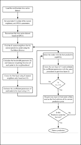
Fig. 2 presents the computation procedure of the proposed method.

e = 1

∑ wi ( yi − yˆi )

i =1

(15)

International Journal of Scientific & Engineering Research, Volume 4, Issue 8, August-2013 1220

ISSN 2229-5518

tem as density and distribution of data points are unlikely to be identical very place of the data set [33]. In this paper, we used the weighted distance algorithm which uses the Ma- halanobis distance metric for optimizing the bandwidth (h) to improve the accuracy of our proposed method.
With the Mahalanobis distance metric, the problem of scale and correlation inherent in Euclidean distance are no longer an issue. In the Euclidean distance, the set of points which have equal distance from a given location is a sphere. The Ma- halanobis distance metric stretches this sphere correct for the respective scales of the different variables.
The standard Mahalanobis distance metric can be defined
as:

d ( x) =

( x − µ )T S −1 ( x − µ )

(19)
where x is the vector of data, µ is a mean and verse covariance matrix.

S −1

is in-
Defining the Mahalanobis distance metric between the
query point xq and data point x as

d q =

( x − xq )

S −1 (

x − xq )

where x belongs to the K nearest neighbors of the query point

xq and

S −1 is computed after removing the main form each-

column, the bandwidth is hq the function of dq :

hq = Θ(d q )

(20)
where

d min ≤ d q ≤ d max and

d min is the distance between

xq and closest neighbor whileis d maxis the distance between

xq and the farthest neighbor.

According to the LWR method, the query corresponding to

d q = d min is most important that is

hmax = θ (d min ) = 1

while
the query point corresponding to

d q = d max

is the least im-

portant, that is hmin = θ (dmax ) = δ ⋅ δ is a real constant. This con-

stant is a low sensitivity parameter. Therefore after few trails,
we fix it to 0.01 which gives the best results.

Fig. 2. Flowchart of the proposed method

The bandwidth hqcan be selected as a function of lows [33]:

d q as fol-

1 − bd q

5 WEIGHTED DISTANCE ALGORITHM FOR OPTIMIZING

THE BANDWIDTH

hq = Θ(d q ) = a (

d q

) + c

(21)
The weighting function bandwidth (h) is a very important parameter which plays an important role in local modeling. If h is infinite then the local modeling becomes global. On the
where a, b and c are constants. By applying the boundary con-
ditions, we can calculate these constants and get [33]:

other hand, if h is too small, then it is possible that we will not
 d
h = (1 − δ )  min
(d max
− d ) 
 + δ
(22)
have an adequate number of data points in the neighborhood for a good prediction.

q 

 q max
− d min 
There are several ways to use this parameter like, constant bandwidth selection, nearest neighbor bandwidth selection where h is set to be a distance between the query point and the
The Gaussian kernel weighting function which used in this paper can be written as following:

Kth nearest point, global bandwidth selection where h is calcu-

lated globally by an optimization process, etc [32].
The constant bandwidth selection method where training data with constant size and shape are used is the easiest and common way to adjust the radius of the weighting function. However, its performance is unsatisfactory for nonlinear sys-

w = exp (− dq )

(23)

International Journal of Scientific & Engineering Research, Volume 4, Issue 8, August-2013 1221

ISSN 2229-5518

6 EXPREMENT RESULTS

6.1 Data

To evaluate the performance of the proposed method, it has been tested for wind power prediction using the real data from wind farms in Alberta, Canada [34]. Alberta has the highest percentage of total installed wind generation capacity of any province in Canada. There are more than 40 wind pro- jects proposed for future development in Alberta. Alberta in- cludes many wind farms such as Ghost pine wind farm (own- ing 51 turbines and 81.6 MW total capacity), Taber wind farm (owning 37 turbines and 81.4 MW total capacity), Wintering Hills wind farm (owning 55 turbines and 88 MW total capaci- ty), etc [35]. The total wind power installed capacity in 2011 is
800MW. This value will be raised to 893 MW by the most re- sent governmental goals for the wind sector in 2012 [35].

6.2 Parameters

To implement a good model, there are some important pa- rameters to choose. There are two important parameters in the KPCA algorithm which used to reconstruct the phase space these parameters are the number of principal components (nc ) and w2 in the Gaussian kernel function. The optimal values of these parameters which computed using the cross validation method are w2=1.9 and nc =10.

In the local prediction model, choosing the neighborhood size (K) is very important step. So, this parameters is calculat- ed as describe in [27] where kmax and β are always fixed for all test cases at 45% of N and 80, respectively.

6.3 Forcasting Accuracy Evaluation

For all performed experiments, we quantified the predic- tion performance with root mean square error (RMSE) and normalized mean absolute error (NMAE) criterion. They can be defined as:
values are used for validation). The length of the forecast hori- zon for the Alberta dataset is 24 hours. Four test weeks (Mon- day to Sunday) corresponding to four seasons of year 2011 are randomly selected for this numerical experiment. These test weeks are: the second week of February 2011 as a winter week, the third week of May 2011 as a spring week, the second week of August 2011 as a summer wee, and the first week No- vember 2011 as a fall week.
The error (RMSE) and (NMAE) of each day during each testing week is calculated. Then the average error of each test- ing week (Monday to Sunday) is calculated by averaging the seven error values of its corresponding forecast days. Finally, the overall mean performance for the four testing weeks for each method can be calculated.
Table 1 shows a comparison between the proposed LWGMDH method and three other approaches (persistence, SARIMA and LRBF), reading the RMSE criterion. These re- sults show that the proposed method outperforms other methods. Table 2 shows the RMSE improvements of the LWGMDH method over persistence, SARIME and LRBF. Ta- ble 3 shows a comparison between the proposed LWGMDH method and three other approaches (persistence, SARIMA and LRBF), regarding the NMAE criterion. These results show the superiority of the proposed method over other methods. Table
4 shows the NMAE improvements of the LWGMDH method over persistence, SARIMA and LRBF.

TABLE 1

COMPARATIVE RMSE RESULTS

1 N

RMSE =

N ∑[ pˆ h − ph ]
(24)

h =1

1 N

TABLE 2

NMAE =

∑ pˆ h − ph ×100

h =1

(25)

IMPROVEMENT OF THE LWGMDH OVER OTHER APPROACHES

REGARDING RMSE

where

pˆ h and

ph are forecasted and actual electricity prices at

hour h, respectively,

pinst is the installed wind power capacity

and N is the number of forecasted hours.

6.4 Results and Discussion

The proposed LWGMDH method has been applied for the prediction of the whole wind power in Alberta, Canada. The performance of the proposed method in compared with 3 pub- lished approaches employing the same dataset. These ap- proaches are resistance, seasonal ARIMA (SARIMA) and local radial basis function (LRBF). Historical wind power data are the only inputs for training the proposed method. For the sake of clear comparison, no exogenous variables are considered.
The proposed LWGMDH method predicts the value of the wind power subseries for one day ahead, taking into account the wind power data of the previous 3 months (the first 80% values of these data are used for training, while the last 20%

TABLE 3

COMPARATIVE NMAE RESULTS

International Journal of Scientific & Engineering Research, Volume 4, Issue 8, August-2013 1222

ISSN 2229-5518

TABLE 4

IMPROVEMENT OF THE LWGMDH OVER OTHER APPROACHES

REGARDING NMAE

	Average RMSE	Improvement
LWGMDH	1.99	--
Persistence	8.21	75.76%
SARIMA	4.17	52.28%
LRBF	2.54	21.65%

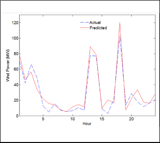
Figs. 3- 6 show the predicted hourly wind power versus the actual wind power of one day (as an example) of each testing week using the proposed LWGMDH method. These results show that our prediction values are very close to the actual values.

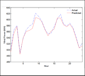
Fig. 5 Forecasted and actual hourly wind power for August 11, 2011

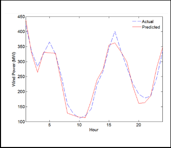
Fig. 3 Forecasted and actual hourly wind power for February 9, 2011

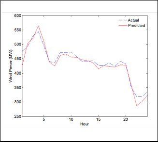
Fig. 6 Forecasted and actual hourly wind power for November 3, 2011

Fig. 4 Forecasted and actual hourly wind power for May 17, 2011

The above results indicate that the proposed LWGMDH method is less sensitivity to the wind power volatility than the other techniques used in the comparison.
To further study the superiority of LWGMDH method, it is also executed for all 52 weeks of year 2011 for the Alberta da- taset and compared with three other approaches (Persistence, SARIMA and LRBF). The results show that the proposed LWGMDH method improves the RMSE and NMAE for the 52 weeks of year 2011 over the Persistence, SARIMA and LRBF methods.
Table 5 shows the RMSE and NMAE improvements of the LWGMDH method over Persistence, SARIMA and LRBF. In addition, Fig. 7 shows the comparison between LWGMDH method and Persistence, SARIMA and LRBF methods for each

International Journal of Scientific & Engineering Research, Volume 4, Issue 8, August-2013 1223

ISSN 2229-5518

month of year 2011 regarding RMSE criterion. Same results can be got using the NMAE criterion.
These results show the robustness of the proposed LWGMDH method and its performance in a long run for a complete year.

TABLE 5

IMPROVEMENT OF THE LWGMDH OVER OTHER APPROACHES

FOR ALL 52 WEEKS OF YEAR 2011

	RMSE Improvement	NMAE Improve- ment
LWGMDH	--	--
Persistence	73.88%	75.35%
SARIMA	51.19%	51.81%
LRBF	20.29%	21.01%

Fig. 7 RMSE Results for the Year Of 2011

7 CONCLUSION

In this paper, we have proposed a LWGMDH based KPCA method for wind power prediction. In the proposed method, the KPCA method is used to reconstruct the time series phase space and the neighboring points are presented by Euclidian distance for each query point. These neighboring points only can be used to train the GMDH where the coefficient parame ers are calculated using the weighted least square (WLS) regres- sion. In addition, the weighting function’s bandwidth which plays a very important role in local modelling is optimized by the weighted distance algorithm.
By using the KPCA the drawback of the traditional time series reconstruction techniques can be avoided by decreasing the correlation between different features in reconstructed phase space. Also, by combining GMDH with the local regres- sion method the drawbacks of global methods can be over- come. In addition, by using the WLS, each point in the neigh- borhood is weighted according to its distance from the current query point. The points that are close to the current query point have larger weights than others. Moreover, by using the weighted distance algorithm, the disadvantage of using the weighting functions bandwidth as a fixed value can be over-
come. This has led to improve the accuracy of the proposed model.
A real world dataset has been used to evaluate the perfor- mance of the proposed model which has been compared with Persistence, SARIMA and LRBF methods. The numerical re- sults show the superiority of the proposed model over Persis- tence, SARIMA and LRBF methods based on different measur- ing errors.

ACKNOWLEDGMENT

The authors gratefully acknowledge the Taif University for its support to carryout this work. It funded this project with a fund number 2742-434-1.

REFERENCES

[1] M. Mazadi, et al., “Impact of Wind Integration on Electricity Markets: a Chance-constrained Nash Cournot Model,” Int. Trans. on Electrical Energy Systems, vol. 23, no. 1, pp. 83–96, 2013.

[2] M. Khalid and A. Savkin, “A Method for Short-term Wind Power Prediction with Multiple Observation Points,” IEEE Trans. Power Systems, vol. 27, no. 2, pp. 579–586, 2012.

[3] H.M. I. Pousinho, V.M.F. Mendes, and J.P S. Catalo, “A hybrid PSO ANFIS Approach for Short-term Wind Power Prediction in Portugal,” Energy Con- version and Management, (In press.)

[4] M. Negnevitsky, P. Mandal, and A.K. Srivastava, “Machine Learning Appli- cations for Load, Price and Wind Power Prediction in Power Systems,” Proc. of 15th Int. Conf. on Intelligent Syst. Appl. to Power Syst., Nov.8–12, pp. 1–6,

2009.

[5] L. Wang, L. Dong, Y. Hao, and X. Liao, “Wind Power Prediction Using Wave- let Transform and Chaotic Characteristics,” Proc. of World Non-Grid- Connected Wind Power and Energy Conf., (WNWEC 2009), Sept.24–26, pp.

1–5, 2009.

[6] L. Ma, et al., “A Review on the Forecasting of Wind Speed and Generated

Power,” Renew. Sust. Energy Rev., vol. 13, no. 4, pp. 915–920, May 2009.

[7] G. Sideratos and N. Hatziargyriou, “Using Radial Basis Neural Networks to Estimate Wind Power Production,” Proc. of Power Eng. Soc. General Meet- ing, Tampa, FL, June24–28, pp. 1–7, 2007.

[8] W. Jiang, Z. Yan, D. Feng, and Z. Hu, “Wind Speed Forecasting Using Auto- Regressive Moving Average/Generalized Autoregressive Conditional Heter- oscedasticity Model,” European Transactions on Electrical Power, vol. 22, no.

5, pp. 662–673, 2012.

[9] R.G. Kavasseri and K. Seetharaman, “Day-ahead Wind Speed Forecasting

Using F-ARIMA Models,” Renew. Energy, vol. 34, no. 5, pp. 1388–1393, May

2009.

[10] N. Amjady, F. Keynia, and H. Zareipour, “Wind Power Prediction by a New Forecast Engine Composed of Modified Hybrid Neural Network and En- hanced Particle Swarm Optimization,” IEEE Trans. Sustainable Energy, vol. 2, no. 3, pp. 265–276, 2011.

[11] K. Bhaskar and S. Singh, “AWNN-assisted Wind Power Forecasting Using

Feed-Forward Neural Network,” IEEE Trans. Sustainable Energy, vol. 3, no.

2, pp. 306–315, 2012.

[12] C.W. Potter and W. Negnevitsky, “Very Short-term Wind Forecasting for

Tasmanian Power Generation,” IEEE Trans. Power Syst., vol. 21, no. 2, pp.

965–972, May 2006.

[13] N. Amjady, F. Keynia, and H. Zareipour, “A New Hybrid Iterative Method for Short-term Wind Speed Forecasting,” European Transactions on Electrical

International Journal of Scientific & Engineering Research, Volume 4, Issue 8, August-2013 1224

ISSN 2229-5518

Power, vol. 21, no. 1, pp. 581–595, 2011.

[14] S. Fan, et al., “Forecasting the Wind Generation Using a Two-stage Network Based on Meteorological Information,” IEEE Trans. Energy Convers., vol. 24, no. 2, pp. 474–482, 2009.

[15] A. J. Smola and B. Scholkopf, “A Tutorial on Support Vector Regression,” NeuroCOLT Technical Report NC-TR-98-030, Royal Holloway College, Uni- versity of London, 1998.

[16] D. Ying, J. Lu, and Q. Li, “Short-Term Wind Speed Forecasting of Wind Farm Based on Least Square-support Vector Machine,” Power Syst. Technology, vol. 32, no. 15, pp. 62–66, Aug. 2008.

[17] M. Zhang, “Short-term Load Forecasting Based on Support Vector Machines

Regression,” Proc. of the Fourth Int. Conf. on Machine Learning and Cyber.,

2005.

[18] A.G. Ivakhnenko, “Polynomial Theory of Complex Systems,” IEEE Trans. of

Syst., Man and Cyber., vol. SMC-1, pp. 364–378, 1971.

[19] S.J. Farlow, “Self-organizing Method in Modeling: GMDH Type Algorithm, Marcel Dekker Inc., 1984.

[20] D. Srinivasan, “Energy Demand Prediction Using GMDH Networks,” Neu- rocomputing, vol. 72, pp. 625–629, 2008.

[21] R.E. Abdel-Aal, M.A. Elhadidy, and S.M. Shaahid, “Modeling and Forecast- ing the Mean Hourly Wind Speed Time Series Using GMDH-based Abduc- tive Networks,” Renewable Energy, vol. 34, no. 7, pp. 1686–1699, 2009.

[22] E.E. El-Attar, J.Y. Goulermas, and Q.H. Wu, “Forecasting Electric Daily Peak Load Based on Local Prediction,” Proc. IEEE Power Engineering Society Gen- eral Meeting (PESGM09), pp. 1–6, 2009.

[23] F. Takens, “Detecting Strange Attractors in Turbulence,” Lect. Notes in Math-

ematics (Springer Berlin), vol. 898, pp. 366–381, 1981.

[24] D. Tao and X. Hongfei, “Chaotic Time Series Prediction Based on Radial Basis Function Network,” Proc. Eighth ACIS Int. Conf. on Software Engin., Artifi- cial Intelligence, Networking, and Parallel/Distributed Computing, pp. 595–

599, 2007.

[25] L. Caoa, et al., “A comparison of PCA, KPCA and ICA for Dimensionality

Reduction in Support Vector Machine,” Neurocomputing, vol. 55, pp. 321–

336, 2003.

[26] F. Chen and C. Han, “Time Series Forecasting Based on Wavelet KPCA and Support Vector Machine,” Proc. IEEE Int. Conf. on Automation and Logistics, pp. 1487–1491, 2007.

[27] E.E. Elattar, J.Y. Goulermas, and Q.H. Wu, “Electric Load Forecasting Based

on Locally Weighted Support Vector Regression,” IEEE Trans. Syst., Man and

Cyber. C, Appl. and Rev., vol. 40, no. 4, pp. 438–447, 2010.

[28] E.E. Elattar, J.Y. Goulermas, and Q.H. Wu, “Integrating KPCA and Locally Weighted Support Vector Regression for Short-term Load Forecasting,” Proc. the 15th IEEE Miditerranean Electrotechnical Conf. (MELECOn 2010), Vallet- ta, Malta, Apr. 25–28, pp. 1528–1533, 2010.

[29] J. Xi and M. Han, “Reduction of the Multivariate Input Dimension Using Principal Component Analysis,” Lect. Notes in Computer Science, vol. 4099, pp. 366–381, 2006.

[30] S. Haykin, “Neural networks: A Comprehensive Foundation”, Printic-Hall,

Inc., 1999.

[31] A.G. Ivakhnenko and G.A. Ivakhnenko, “The Review of Problems Solved by Algorithms of the Group Method of Data Handling (GMDH),” Pattern Recognition and Image Analysis, vol. 5, pp. 527–535, 1995.

[32] C.C. Atkeson, A.W. Moore, and S. Schaal, “Locally Weighted Learning,” Artificial Intelligence Review (Special Issue on Lazy Learning), vol. 11, pp. 11–

73, 1997.

[33] H. Wang, C. Cao, and H. Leung, “An Improved Locally Weighted Regression for a Converter Re-vanadium Prediction Modeling,” Proc. the 6th World Congress on Intelligent Control and Automation, pp. 1515–1519, 2006.

[34] Alberta Electric System Operator (AESO), Wind Power tion http://www.aeso.ca/gridoperations/13902.htm l. (2013)

[35] Canadian Wind Power Association

WEA). http://www.canwea.ca/farms/wind-farms e.php. (2013)