International Journal of Scientific & Engineering Research, Volume 6, Issue 3, March-2015 641
ISSN 2229-5518
General method for data indexing using clustering methods
Karwan Jacksi, Sobhan Badiozamany
Abstract— Indexing data plays a key role in data retrieval and search. New indexing techniques are proposed frequently to improve search performance. Some data clustering methods are previously used for data indexing in data warehouses. In this paper, we discuss general concepts of data indexing, and clustering methods that are based on representatives. Then we present a general theme for indexing using clustering methods. There are two main processing schemes in databases, Online Transaction Processing (OLTP) and Online Analytical Processing (OLAP). The proposed method is specific to stationary data like in OLAP. Having general indexing theme, different clustering methods are compared. Here we studied three representative based clustering methods; standard K-Means, Self Organizing Map (SOM) and Growing Neural Gas (GNG). Our study shows that in this context, GNG out performs K-Means and SOM.
Index Terms— Clustering Algorithms, K-Means, Self Organizing Map (SOM), Growing Neural Gas (GNG), Database Indexing.
—————————— ——————————
1 INTRODUCTION
e review general database indexing concepts in sec- tion 1.1. Then we cover spatial indexing concepts and methods in section 1.2. Clustering methods that are
based on representatives are discussed in section 1.3.
1.1 Database indexing general concepts
Database Indexes are supplementary access structures which are used to make the search faster when looking up for rec- ords. Indexes provide secondary access path to data files, meaning that they do not alter the placement of records in the main data file. Index can be put on any data field (attribute), there could be more than one index per single data file. Index can also be defined on a combination of attributes. Index files are usually have two fields, <Key, pointer>, where key is the value of indexing attribute and the pointer is the physical address for records having a certain value in their index field.
Having indexes as an extra access path, the search is done in two steps, first accessing the index structure looking up for the key, then following the pointer in the index entry to get to the actual record in data file.
The most common indexing methods are B+-trees and hashing indexes. B+-trees are the most common structure for generating indexes in most relational Database Management Systems (DBMSs) (1).
1.2 Spatial indexing methods
Many scientific applications produce multidimensional spatial datasets that are very huge, both dimensionally and vertically. The fact that conventional database indexing techniques are
————————————————
• Karwan Jacksi is currently pursuing PhD degree program in Computer Science in University of Zakho, Iraq and Eastern Mediterranean Univerisy, Cyprus. Tel: +90-533-852-8257. Email: Karwan.Jacksi@uoz.ac
• Sobhan Badiozamany is currently pursuing PhD degree program in Com-
puter Science in Uppsala University, Sweden, Tel: +4670-4094664, Email: sobhan.badiozaman@gmail.com
unable to index spatial datasets caused huge efforts in making specific indexing techniques for spatial datasets.
Spatial indexing methods can be grouped into two sets; space partitioning methods and data partitioning methods. Space partitioning methods that are based on KD-trees (2) have been shown to perform well for point data. In space par- titioning, we start by inserting elements into tree. When over- flow happens, a single dimension and a single position in that dimension are used to split nodes. Data partitioning methods, based on R-trees split the space using rectangular bounding boxes. The positions of bounding boxes are stored in the index structure (3).
1.3 Clustering General Concepts
Clustering divides data into groups (clusters) based on the similarity between data points. The aim of grouping is either to divide data into meaningful groups or as a preprocessing step, for instance to summarize data. In case the clustering intention is to find meaningfulness of data, so called natural clusters are generated by clustering algorithms (4).
There are varieties of clustering algorithms in literature; here we focus on clustering methods that are based on having one or more representatives for each cluster. More specifically, we focus on K-means, Self Organizing Map (SOM) and Grow- ing Neural Gas (GNG).
1.3.1 K-Means
K-means algorithm is one of the simplest clustering methods (4). K initial centroids (or codebooks) are chosen, where K is the parameter to the algorithm (the number of clusters). Each data point is then assigned to the closest centroid. Then the centroid of each cluster is updated based on the mean (aver- age) of all data points in the cluster. The assignment and up- dating steps are repeated until convergence.
K-means is described in more details in the following algo- rithm (4).
• Select K initial centroids
• Repeat
o Form K clusters by assigning each data point
IJSER © 2015 http://www.ijser.org
International Journal of Scientific & Engineering Research, Volume 6, Issue 3, March-2015 642
ISSN 2229-5518
to its closest centroid.
o Recalculate the centroid for each cluster.
• Until centroids do not change.
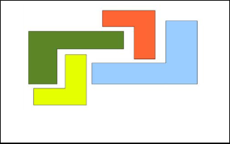
The main advantage of the algorithm is in its simplicity, while the main disadvantage is sensitivity to initialization of K centroids, in that some centroids will not be used while some represent more than one natural cluster. In addition, K-means does not perform well when there is noise (outliers). Further- more, K-Means fails to form natural clusters when clusters have none globular shapes. Figure 1 illustrates an example in which K-means has problems to identify.
Fig. 1. Example of clustering task that K-Means fails to identify.
K-means could be thought of as a version of standard com- petitive learning in which the centroids compete with each other for an input pattern, only the winner (the closest cen- troid) moves toward the input.
1.3.2 Self Organizing Map (SOM)
A Self Organizing Map (SOM) is a grid of artificial neurons that are connected to each other locally. The input vector is connected to all of the nodes on the grid. Therefore, it could be imagined as each node on the grid has a position in the input space, defined by its weight vector. Only one cell (or group of neighboring cells) reacts to a given input vector at a time (5). The learning is unsupervised and is a version of competitive learning that is extended to move not only the winner, but also the nodes that are neighbors to the winner on the grid. The following algorithm explains how the learning happens in SOM (5).
• Initialize the network.
• Repeat
o Present the input vector x.
o For each node, j, compute the distance, d, between
its weight vector and the input vector:
o Find the node, k, which is closest to the current input vector.
o Update the weights of all nodes by
Wji = Wji + ηf(j,k)(Xi – Wji)
Where η is the learning rate and f(j,k) is the neighborhood function
SOM is a dimension reduction method, since it maps the input data which (usually) has higher dimensionality, to (usu-
ally) 2D grid. As a result of update rule in the algorithm, the groups of nodes that are close on the map react to similar in- put patterns. This results in a topologically preserving map.
The main advantage of SOM is that it builds up a topologi- cally preserving map of the input data. In addition, since nodes move together, SOM is not sensitive to initialization.
1.3.3 Growing Neural Gas (GNG)
Growing Neural Gas (GNG) is an unsupervised growing algo- rithm for clustering. It creates a graph, or network of nodes, incrementally, where each node in the graph has a position in N-dimensional input space.
Centroids in GNG are represented by the reference vectors (the position) of the nodes. GNG preserves topological distri- bution of input data. If the distribution of input data changes over time, GNG is able to adapt, that is to move the nodes so as to cover the new distribution.
The GNG algorithm can be summarized as following (6).
• Start with two nodes at random position.
• For each input vector x
o Find the closest node, the winner (k), and the se-
cond closest (r).
o Move the winner k, and its neighbors n by;
∆Wk = εk (X − Wk) ∆Wn = εn (X − Wn)
Where, W is the node position (its weight vector) and both εk and εn (gain factors) are constant.
o If k and r are not already connected (neighbors), connect them with a new edge.
o Set the age of the edge between k and r to 0.
o Increment the age of all other edges emanating
from k by one.
o Remove the edge when it becomes too old (> age max).
o Remove the node if it loses its last edge this way.
• When a winner, k, is found, add the distance from the input
vector to a local error variable.
• Insert a new node halfway between the node with the larg-
est error, and the node among its current neighbors with the largest error.
• Decay the error of a node over time
The main advantages of GNG is that, it has dynamic size which can grow or shrink, dynamic neighborhood means there is no fixed neighbors; instead neighbors are defined by the graph. All parameters are constant; there is no decaying parameter, which is great for on-line learning.
2 RELATED WORKS
SOMs are used in physical data warehouse design (7). Data warehouses are built for Online Analytical Processing (OLAP), where the main aim is data reporting and analysis (8). There- fore they are not updated as frequently as Online Transaction Processing (OLTP) databases. Since OLAP is mainly used for reporting and analysis, fast retrieval of data is of high de- mand. In contrast with OLTP where data is stored in tables, OLAP usually stores data in multidimensional arrays usually called cubes. Array indexes provide automatic indexing meth-
IJSER © 2015 http://www.ijser.org
International Journal of Scientific & Engineering Research, Volume 6, Issue 3, March-2015 643
ISSN 2229-5518
od for multidimensional data. Having an automatic indexing structure, now the main problem is how to map dimension attribute values to indexes. Figure 21 illustrates how multidi- mensional data is stored in an array.
In this method, In order to build the index structure, data has to be clustered first. After the clustering is done, each rep- resentative becomes an index entry in the index structure, pointing to the set of disk blocks that contain data records of that cluster.
Figure 3 illustrates a very simple clustering of 12 data points. There are 3 representatives, c1, c2 and c3, one per each cluster.
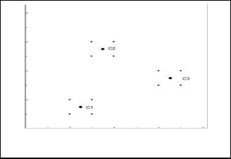
Fig. 2. Multidimensional data cube
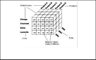
SOM can be used for this purpose. Consider that we have a data cube with three dimensions: region, date and product, and one measure: sales amount. For example, one cell in this cube can be addressed as [China][2009][Chair] and the content of this cell reveals the sales amount. This specific cell is stored in a certain position in multidimensional array, for example [2][4][25], where ‘China’ is indexed to 2, ‘2009’ indexed to 4 and ‘Chair’ indexed to 25.
As proposed in (7), single SOM can be used in each dimen- sion to map dimension attributes to index numbers. The at- tribute values are the input to SOM and index of the active node on the grid is the index for specific attribute value. For instance the SOM for region dimension maps ‘China’ to 2, because ‘China’ activates 2nd node on the grid. Dimension values like ‘2009’ and ‘Chair’ are mapped to 4 and 25 in the same way.
The main advantage of using SOM for indexing multidi- mensional data is its capability of detecting misspellings, for example it is likely that ‘Shina’ is also indexed to 2. In common database indexing methods every key value is mapped to one specific point in the space, while in SOM based indexing, be- cause of SOM’s generalization ability, every key value is mapped to a region in the space.
When SOM is used for indexing, to find the index value of a given input, the closest node has to be identified. This could become very costly when the number of nodes increases. Spa- tial indexing methods are proposed (9) (10) as an extra level of indexing to speed up the overall search time.
3 GENERAL THEME FOR INDEXING DATA USING CLUSTERING METHODS
So far we have discussed three clustering methods, K- Means, SOM and GNG. The common characteristic between all of them is that they use one or more representatives to identify each cluster. In this section, we show that data can be indexed using any clustering method that is based on repre- sentatives.
1 The figure is from (7).
Fig. 3. Simple Clustering.
The centroid C1= (1.25, 0.75), C2= (1.75, 2.75) and C3= (3.25,
1.75) will be the keys in the index structure, each one pointing
to one (or more, if there are too many nodes in the cluster)

disk block. The index structure looks like the Figure 4.
Fig. 4. Proposed index structure.s
Depending on the density of data in each cluster, in some cases there will be too many data points in each cluster, mak- ing it impossible to fit all of them in a single disk block. There are two main approaches to resolve this issue. First solution is to use clustering methods that put more representatives where the density is higher. The second approach is usually called chaining, where a single index entry is used for the dense cluster which points to the first disk block containing cluster record. In latter scheme each disk block contains a pointer to the next disk block in the chain.
Since a linear search has to be done in the indexing file in order to find the closest centroid to a given input, if the num- ber of centroids increases, the search will be costly. Spatial
IJSER © 2015 http://www.ijser.org
International Journal of Scientific & Engineering Research, Volume 6, Issue 3, March-2015 644
ISSN 2229-5518
indexing methods can be employed, as a top level index when looking for closest centroid. This improves the scalability of proposed indexing method (9) (10).
4 CLUSTERING METHODS COMPARISON FOR INDEXING
Since the general theme for indexing data is dependent on how representatives are distributed in the input space, the clustering algorithms that can distribute them more evenly are recommended. For instance, since some centroids are not used in standard K-Means, indexing structure built on K-Means is more likely to get the problem of having too many data points per some representatives (index entries). The same problem, but with a lower severity can happen for SOM because there are some nodes on the grid that are not presenting cluster. In contrast, GNG outperforms both K-Means and SOM since it grows dynamically and covers more dense areas with more representatives.
Another factor is the computation cost of clustering algo- rithms. Since clustering has to be done as a prerequisite for indexing, clustering performance has to be taken into account when the overall indexing performance is compared.
5 CONCLUSION AND FUTURE WORK
We have shown how clustering methods that are based on representatives can be used for indexing. The clustering meth- ods that distribute representatives more evenly in clusters perform better in the proposed schema. Out of the clustering methods we studies, GNG was the best for indexing. As an extra level of indexing, spatial indexing, like R-tree, can be used to improve overall performance of indexing.
The proposed indexing method performs well when data distribution is fixed. In other words, when there is no modifi- cation to database (insert/update/delete). One possible appli- cation of these methods is OLAP where data is never updated. If the data distribution changes, centroids start moving, and every time they change position, data points have to be redis- tributed among them, which decrease the indexing algorithms performance dramatically. Further studies are required to extend this method to deal with database modifications.
Furthermore, practical experiments need to be done to compare the performance of this indexing method with com- mon indexing methods.
REFERENCES
[1] 1. Ramez Elmasri, Shamkant B. Navathe. Fundamentals of Database Systems.
Fundamentals of Database Systems. s.l. : Pearson Education, Limited, 2013,
2013, pp. 455-493.
[2] 2. Multidimensional Binary Search Trees used for associative searching.
Bently, J.L. 1975, Communications of ACM .
[3] 3. A Comparative Study of Spatial Indexing Techniques for Multidimensional
. Sussman, Beomseok Nam and Alan. 2004, MISC.
[4] 4. Tan, Pang-Ning, Michael Steinbach, and Vipin Kumar. Introduction to Data
Mining. In Introduction to Data Mining . s.l. : Addison-Wesley, 2006. [5] 5. The Slef Organizing Map. Kohonen, Teuvo. 1990, IEEE.
[6] 6. A growing neural gas network learns topologies. Fritzke, Bernd. 1995, (MIT
Press) Advances in neural information processing systems 7 .
[7] 7. PHYSICAL DATA WAREHOUSE DESIGN USING NEURAL . Sharma, Mayank, Navin Rajpal, and B.V.R.Reddy. 2010, (International Journal of Computer Applications) 1 .
[8] 8. OLAP, Wikipedia. [Online] Wikipedia, 11 11, 2014. [Cited: November 11,
2014.] https://en.wikipedia.org/wiki/Online_analytical_processing.
[9] 9. A SAM-SOM Family: Incorporating Spatial Access Methods into Construc- tive Self-Organizing Maps . Vargas, Ernesto Cuadros, and Roseli A. Francelin Romero. 2002, MISC.
[10] 10. Cuadros-vargas, Ernesto, Roseli Ap, Francelin Romero, and Klaus Ober- mayer. Speeding up algorithms of SOM Family for Large and High Dimen- sional Databases. s.l. : In Workshop on Self organizing Maps, 2003.
IJSER © 2015 http://www.ijser.org