INTRODUCTION
T
he speaker recognition has always focused on security system of controlling the access to control data or infor-
mation being accessed by any one. Speaker recognition is the process of automatically recognizing the speaker voice according to the basis of individual information in the voice waves. Speaker identification is the process of using the voice of speaker to verify their identity and control acess to services such as voice dialing, mobile banking, data base acess services, voice mail or security control to a secured system.
The recognition and classification of audio information have multiple applications [1].The identification of the audio context for portable devices, which could allow the device to automatically adapt to the surrounding environment without human intervention [2]. In robotics this technology might be employed to make the robot interact with the environment, even in the absence off light, and there are surveillance and security system that make use of the audio information either by itself or in combination with video information [1].
PRINCIPLE OF VOICE RECOGNITION
Speaker Recognition Algorithms
A voice analysis is done after taking an input through micro- phone from a user. The design of the system involves manipu- lation of the input audio signal. At different levels, different operations are performed on the input signal such as Window- ing, Fast Fourier Transform, GT Filter Bank, Log function and discrete cosine transform.
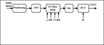
The speaker algorithms consist of two distinguished phases. The first one is training sessions, whilst, the second one is re- ferred to as operation session or testing phase as described in figure 1[3].
Fig.1. Speaker Recognition algorithms
Gammatone Filter Properties
Gammatone function models the human auditory filter re- sponse. The correlation between the impulse response of the gammatone filter and the one obtained from the mammals was demonstrated in [8]. It is observed that the properties of frequency selectivity of the cochlea and those psychophysiclly measured in human beings seems to converge, since: 1) the magnitude response of a fourth-order GT filter is very similar to reox function [7], and 2) the filter bandwidth corresponds to a fixed distance on the basilar membrane. An nth-order GT filter can be approximated by a set of n first-order GT filter placed in cascade, which have an efficient digital implementa- tion.
Gammatone Cepstral Coefficients
Gammatone cepstral coefficients computation process is anal- ogous to MFCC extraction scheme. The audio signal is first windowed into short frames, usually of 10–50 ms. This process has a twofold purpose 1) the (typically) non-stationary audio signal can be assumed to be stationary for such a short inter- val, thus facilitating the spectro-temporal signal analysis; and
2) the efficiency of the feature extraction process is increased
IJSER © 2013
[1]. Subsequently, the GT filter bank (composed of the fre- quency responses of the several GT filters) is applied to the signal’s fast Fourier transform (FFT), emphasizing the percep- tually meaningful sound signal frequencies.1 Indeed, the de- sign of the GT filter bank is the object of study in this work, taking into account characteristics such as: total filter bank bandwidth, GT filter order, ERB model (Lyon, Greenwood, or Glasberg and Moore), and number of filters. Finally, the log function and the discrete cosine transform (DCT) are applied to model the human loudness perception and decorrelate the logarithmic-compressed filter outputs, thus yielding better energy compaction. The overall computation cost is almost equal tothe MFCC computation [6].
form (FFT), emphasizing the perceptually meaningful sound signal frequencies [6].
Fig.2. Block diagram describing the computation of the adapted Gamma- tone cepstral coefficients, where stands for the GT filter order, the filter bank bandwidth, the equivalent rectangular bandwidth model, the number of GT filters, and for the number of cepstral coefficients.
Feature Extraction
The extraction of the best parametric representation of acous- tic signals is an important task to produce a better recognition perfomance. The efficiency of this phase is important for the next phase since it affects its behavior.
Step 1: Windowing
The audio samples are first windowed (with a Hamming win-
dow) into 30 ms long frames with an overlap of 15 ms. The frequency range of analysis is set from 20 Hz (minimum audi- ble frequency) to the Nyquist frequency (in this work, 11 KHz). This process has a twofold purpose 1) the (typically) non-stationary audio signal can be assumed to be stationary for such a short interval, thus facilitating the spectro-temporal signal analysis; and 2) the efficiency of the feature extraction process is increased.
The Hamming window equation is given as:
If the window is defined as W (n), 0 ≤ n ≤ N-1 where
N = number of samples in each frame Y[n] = Output signal
X (n) = input signal
W (n) = Hamming window, then the result of windowing sig- nal is shown below:
Y (n) = X (n) * W (n)
W (n) = 0.54 – 0.46 cos [ 2Пn / N-1 ] 0 ≤ n ≤ N – 1
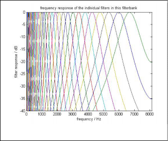
Step 2: GT Filter Bank
The GT filter bank composed of the frequency responses of the
several GT filters. It is applied to the signal’s fast Fourier trans-
Fig.3. Filter Bank output
Step 3: Fast Fourier Transform
To convert each frame of N samples from time domain into
frequency domain.
Y (w) = FFT [h (t) * X (t )] = H (w ) * X(w)
If X (w), H (w) and Y (w) are the Fourier Transform of X (t), H
(t) and Y (t) respectively.
Step 4: Discrete Cosine Transform
The log function and the discrete cosine transform (DCT) are
applied to model the human loudness perception and decorre-
late the logarithmic-compressed filter outputs, thus yielding
METHODOLOGY
Voice recognition works based on the premise that a person voice exhibits characteristics are unique to different speaker. The signal during training and testing session can be greatly different due to many factors such as people voice change with time, health condition (e.g. the speaker has a cold), speaking rate and also acoustical noise and variation record- ing environment via microphone [5]. Table I gives detail in- formation of recording and training session.
Process | Description |
Speaker | Three Female Two Male |
Tools | Mono microphone Matlab software |
Environment | Laboratory |
Sampling Frequency, fs | 8000Khz |
TABLE 1 TRAINING REQUIREMENT
EXPERIMENTAL EVALUATION
Audio Database
Speech samples are taken from five persons. From each person 50 to 60 samples are taken .The length of the speech samples was experimentally set as 4s.
TABLE 2 AUDIO DATABASE
Speaker
Samples
Speaker 1
61
Speaker 2
50
Speaker 3
59
Speaker 4
50
Speaker 5
50
Experimental Setup
The speech samples are first windowed (with a Hamming window) into 30 ms long frames with an overlap of 15 ms, as done in [3]. The frequency range of analysis is set from 20 Hz (minimum audible frequency) to the Nyquist frequency (in this work, 11 KHz). Subsequently, audio samples are parame- terized by means of GTCC (both the proposed adaptation and previous speech-oriented implementations [7]–[9]) and other state-of-the art features (MFCC and MPEG-7). MFCC are computed following their typical implementation [4].With regard to MPEG-7 parameterization, we consider the Audio Spectrum Envelope (since it was the MPEG-7 low level de- scriptor attaining the best performance for non-speech audio recognition in which is converted to decibel scale, then level- normalized with the RMS energy [4], and finally compacted with the DCT.
Rather than performing the audio classification at frame-level, we consider complete audio patterns extracted after analyzing the whole 4 s-sound samples at frame-level. With reference to these kinds of sounds, it is of great relevance to consider the signal time evolution (including envelope shape, periodicity and consistency of temporalchanges across frequency cha- nels). Subsequently, the audio patterns obtained are compact- ed by calculating the mean feature vector over different inter- vals [9]. The main purpose of this process is to make the classi- fication problem affordable without losing the feature space interpretability, which would happen if considering, for ex- ample, principal component analysis or independent compo- nent analysis [3]. This requirement is especially important, since we are mainly interested in determining the rationale behind the performance of GTCC in contrast to other state-of- the-art audio features.
Regarding the classification system, three machine learning methods are used for completeness: 1) a neural network (NN), and more specifically, a multilayer perceptron with one hid- den layer; and 2) a support vector machine (SVM) with a radi- al basis function kernel and one versus all multiclass approach and K-nearest neighbor [9]. The audio patterns are divided into train and test data sets using a 10 10-fold cross validation scheme to yield statistically reliable results. Within each fold, the samples used for training are different from those used for testing. In addition, the last experiment employs a 4-fold cross validation scheme with a different setup, whose aim is to test the generalization capability of the features. The classification accuracy is computed as the averaged percentage of the test- ing samples co rectly classified by each machine learning method
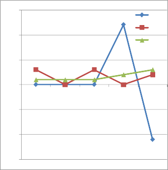
EXPERIMENTAL RESULTS
GTCC Adjustment