International Journal of Scientific & Engineering Research, Volume 5, Issue 2, February-2014 759

ISSN 2229-5518

Finite Difference Scheme for the Zakharov Equation as a Model for Nonlinear Wave- Wave Interaction in Ionic Media

Arun Kumar* and Ram Dayal Pankaj

Abstract: In the paper, the coupled 1D Zakharov Equation (ZE) is considered as the model equation for wave-wave interaction in ionic media. A new six point finite difference scheme, which is equivalent to the multi-symplectic integrator, is derived for the model equations. The numerical simulations are also presented for the model.

Keywords: Zakharov equation, Multi-symplectic scheme; Finite difference scheme, Wave-Wave Interaction,

1. Introduction:

Physically, the wave-wave interaction or the wave collisions are common phenomena in science and engineering for both solitary and non-solitary waves. At the classical level, a set of coupled nonlinear wave equations describing the interaction between high-
frequency Langmuir waves and low-frequency ion-acoustic waves
16]. However in their numerical simulations, in order to keep the accuracy, there are many constraints. In the paper, we discretize the system with finite difference schemes to get the numerical simulations of the ZE

2. A difference scheme for ZE system

Considering the ZE system (1) and taking
were firstly derived by Zakharov [1]. Since then, this system has been the subject of a large number of studies. The system can be
derived from a hydrodynamic description of the plasma [2,3].

E = p ( x, t ) + iq ( x, y ) ,

we get

η = µ ( x, t ) + iξ ( x, y )

However, some important effects such as transit-time damping and ion nonlinearities, which are also implied by the fact that the

qt − pxx = ( qξ − pµ );

pt + qxx = ( pξ + qµ )

values used for the ion damping have been anomalously large

µ − µ

− (( p )2

+( q )2

) = 0;

from the point of view of linear ion-acoustic wave dynamics, have

tt xx

xx xx

(2)
been ignored in the Zakharov Equation (ZE). That is to say, the
ZE is a simplified model of strong Langmuir turbulence. Thus we

ξtt

− ξ xx = 0

have to generalize the ZE by taking more elements into account. Starting from the dynamical plasma equations with the help of
relaxed Zakharov simplification assumptions, and through taking
Introducing the canonical momenta

px = b, qx = a, µx = d ,ζ x = c ,

use of the time-averaged two-time-scale two-fluid plasma

µ = e, ξ

= f , g = ( p2 )

, h = (q2 )

(3)
description, the Zakharov Equations are generalized to contain the

t t x x

The above system can be written in the following form
self-generated magnetic field [4]. The ZE are a set of coupled

Kz + Lz

= ∇ S ( z)

(4)
equations as mentioned in [5]

t x z

Which is a multi-symplectic in nature with the state variables

iEt

+ Exx − nE = 0,

z = (p, q, b, a, µ ,ξ , d , c, e, f , g , h, p 2 , q 2 )T

∈ R14

ntt

− nxx

− E 2 = 0

(1 )
The system is multi-symplectic in the sense that K is a skew- symmetric matrix representative of the t direction and L is a skew-
symmetric matrix representative of the x direction. S represents a
where E is the envelope of the high-frequency electric field, n is
Hamiltonian function, then (2) can be transformed in
the plasma density measured from its equilibrium value. Up to

q − p

= (ξ q − pµ ) ; p + q

= ( pξ + qµ ) ;

now, there are many methods of constructing exact solutions, for instance, the inverse scattering transform [6], the Hirota method
[7], the Backlund method [8], the extended tanh-function method

t xx t xx

px = b ; qx = a, µx = d ; ξ x = c ; µt = e ;

(5)
[9], the variable separation approach [10], the Adomian methods

ξ = f , ( p2 )

= g; (q2 )

= h;

decomposition method [11–13] and several other numerical [14-

t x x

————————————————

µ − µ

− (( p )2

+ ( q )2

) = 0; ξ − ξ

= 0 ;

* Department of Mathematics Government College, Kota, India arunkr71@gmail.com

1 Department of Mathematics

JNV University, Jodhpur, India

tt xx

and

xx xx

tt xx

International Journal of Scientific & Engineering Research, Volume 5, Issue 2, February-2014 760

ISSN 2229-5518

qt − bx = (ξ q − pµ ) ; pt + ax = ( pξ + qµ ) px = b ;

n+1

n n+1 2

n+1 2

qx = a ; et − d x − ( g x + hx ) = 0; ft − cx = 0

(6)

ql +1 2 − ql +1 2 − bl +1

∆t

− bl

∆x

(7)

µx = d ; ξx = c ; µt = e ;

= (ξˆqˆ −

pˆ µˆ )

ξ = f

; ( p2 )

= g ; (q2 ) = h

p n+1

− p n

an+1 2 − an+1 2

t x x

So that

l +1 2

∆t

l +1 2 + l +1 l

∆x

(8)

∇ S (z ) = (kp, kq, b, a, sp, sq, d , c, e, f , g , h, p 2 , q 2 )T

where

kp = (ξ q − pµ ) ;

kq = ( pξ +qµ ) ;

= ( pˆξˆ + qˆ µˆ )

n +12 n +12

l +1 l n +1 2

l +1 2

(9)

px = b ;

qx = a ;

sp = 0 ;

sq = 0;

∆x

n+1 2

µ x = d ; ξ x =

c ; µ

= e ;

ql +1

− ql

∆x

n+1 2

l +1 2

(10)

ξt =

f ; ( p 2 )

= g ; (q 2 ) = h

el +1 2 − el +1 2 d − d

n+1

n n+1 2

l +1

n+1 2

x x

and the pair of skew symmetric matrix K and L are

− −

∆t ∆x

(11)

 g n+1 2 − g n+1 2

hn+1 2 − hn+1 2 

0 1



0 0 0

0 0 0 0 0 0 0

0 0



 l +1 l + l +1 l  = 0

1 0

0 0



0 0 0

0 0 0 0

0 0



 ∆x

n+1 n

∆x

n+1 2



n+1 2

0 0

K= 0 0

0 0 0

0 0 0 0

0 0 0 1

0 0 0

0 0



fl +1 2 −

∆t

fl +1 2

= cl +1

− cl

∆x

(12)

0 0



0 0

0 0 0

0 0 0 0 1 0 0

0 0 0 0 0 0 0

0 0



0 0

n+12

l +1

− µ n+1 2

∆x

n+1 2

l +1 2

(13)

0 0



0 0



0

0 0

0 0 1 0

0 0 0 1

0 0 0 0

0 0 0 0



0 0 0 0

0 0 0 

0 0 0 0

n +12

l +1

µ n +1

− ξ n +1 2

∆x

− µ n

n +1 2

l +1 2

(14)



0 0

0 0

0 0 0

0 0 0 0



0 0 0 0 0

0 0 0 0 

l +1 2

∆t

l +1 2

n +1 2

l +1 2

(15)

0 0 1 0 0 0 0

0 0 0 1 0 0 0

1 0 0 0 0 0 0



0 0 0 0 0 0

0 0 0 0

0 0 0

0 0 

0 0 0



0 0 

n +1

l +1 2

l +1 2 =

∆t

n +1 2

l +1 2

(16)

0

L= 

0

0 0 0 0 0

0 0 0 1 0

− 1 0 0 0

0 1 0 0

0 0 0 0

− 1 − 1 0 0



0 0 0 0

(p 2

n +1 2

l +1 2

∆x

l +1 2

n +1 2

l +1 2



0 0



0 0

0 0 0 1 0

0 0 0 0 0

0 0 0 0



0 0 0



0 0 0

2 n +1

l +1 2

2 n

l +1 2

∆x

n +1 2

l +1 2

  ˆ

n+1 2 , ˆ

n+1 2

0 0 0 0 0 0 0



0 0 0 0

0 1 0

0 0 1



µ = µl +1 2

q = ql +1 2

p = pl +1 2

ξ = ξl +1 2

0 0 0 0 0 0 0

0 0 0 0 0 0 0

0 0 0 0

0 0 0

0 0 

From (7) and (9), we eliminate b, we get
Using midpoint difference scheme to discretize multi-symplectic
ZE system, we get

International Journal of Scientific & Engineering Research, Volume 5, Issue 2, February-2014 761

ISSN 2229-5518

l +1 2

l +3 2

l +3 2 −

( l +2

l +1

l ) ( l +2

l +1 l )

qn+1

− qn

+ qn+1

∆t

− q n

E n+1+2E n+1+ E n+1 − E n

2∆t

+2E n

+ E n

2 ( p n+1 2 − 2 p n+1 2 +

p n+1 2 )

( E n 2 + E n+1)−2( E n 1+ E n+1)+( E n + E n+1)

l + 2

l +1 l

( ∆x )2

(17)

l + l +2

l +

(∆x )2

l +1 l l

1 n n+1

n n+1

= (ξ n+1 2 q n+1 2 − µ n+1 2 p n+1 2 ) +

= (( El +1 2 + El +1 2 )(ηl +1 2 + ηl +1 2 ) +

l +1 2

(22)

(ξ n+1 2 q n+1 2 − η n+1 2 p n+1 2 )

( El +3 2 + El +3 2 )(ηl +3 2 + ηl +31 2 ))

n n+1

l +3 2

Multiply (19) with i and adding Eq. (18) then we can get
From (8), (10), we eliminate a we get

n+2

n+1

n n+1

n+1

n +1

l +1 2

n +1

l +3 2

l +3 2 +

(ηl +1

− 2ηl +1

(∆t )2

+ ηl +1 ) (ηl +2 − 2ηl +1

−

(∆x )2

+ ηl )

−

∆t

 n+1 2

n+1 2

n+1 2 

(23)

2 (q n +1 2 − 2q n +1 2 + q n +1 2 )

 = l +2

− 2 El +1

+ El 

l + 2

l +1 l

( ∆x )2

 (∆x )2



 = 0



= (ξ n+1 2 pn+1 2 + µ n+1 2 qn+1 2 ) +

(18)

3. Numerical simulation

l +1 2

In order to verify numerically whether the proposed methodology leads to higher accuracy, we evaluate the numerical solutions of

(ξ n+1 2 pn+1 2 + µ n+1 2 qn+1 2 )

the ZE (1) with initial conditions

l +3 2

E( x, 0) = r tanh( px) exp[ikx],

Similarly we eliminate e & d, g & h and c & f. So we can get

 µ n+2 − 2µ n+1 + µ n

  µ n+1 − 2µ n+1 + µ n+1 

η ( x, 0) = s + r 2 tanh 2 ( px) / (−4k 2 + 1)

 l +1 l +1 l +1 −  l +2 l +1 l −

 (∆t )2

  (∆x)2 

−4kpr 2 tanh( px)(1 − tanh 2 ( px))

   

ηt ( x, 0) =

(−4k 2 + 1)

 ( p2 )n+1 − 2( p2 )n+1 + ( p2 )n+1

(q2 )n+1 − (q2 )n+1 + (q2 )n+1 

(19)

 l +2 l +1 l + l +2 l +1 l  = 0

p2 (4k 2 −1)

 (∆x)2

(∆x)2 

where r =

, p,k ,s,β are arbitrary constt.

  1+(4k 2 −1)β

 ξ n + 2 − 2ξ n +1 + ξ n 

l +1 l +1 l +1 −

 

 ( ∆t )2 

(20)

 ξ n +1 − 2ξ n +1 + ξ n +1 

l + 2 l +1 l = 0

 

 ( ∆x )2 

Multiply (18) with i and adding (17) we get

(E∗n

+ E∗n+1 ) − 2 ( E∗n

+ E∗n+1 ) + (E∗n + E∗n+1 )

l +2

l +1

(∆x )2

l +1 l l

= − 1 (( E∗

n + E∗

n+1 )(η ∗

n + η ∗

n+1 ) + (21)

4 l +1 2

l +1 2

( ∗ n

∗ n+1 )( ∗ n

∗ n+1 ))

El +3 2

+ El +3 2

ηl +3 2

+ ηl +3 2

Conjugating (21)

International Journal of Scientific & Engineering Research, Volume 5, Issue 2, February-2014 762

ISSN 2229-5518

Fig. 1.(a) The numerical result for

E 2 using (22), (b) the exact

References

[1] Zakharov VE. Collapse of Langmuir waves. Zh Eksp Teor
Fiz 1972;62:1745–51.
[2] Goldman MV. Langmuir wave solitons and spatial collapse in plasma physics. Physica D 1986;18:67–76.
[3] Nicholson DR. Introduction to plasma theory. New York: Wiley; 1983.
[4] Li LH. Langmuir turbulence equations with the self-generated magnetic field. Phys Fluids B 1993;5:350–6.
[5] Malomed B, Anderson D, Lisak M, Quiroga-Teixeiro ML.
Dynamics of solitary waves in the Zakharov model equations. Phys Rev E 1997;55:962–8.
solution for

E 2 with the initial condition (18) when the

[6] Vakhnenko VO, Parkes EJ, Morrison AJ. A Backlund transformation and the inverse scattering transform method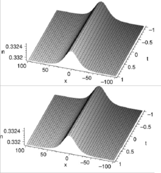

parameters p = 0.05, k = 1, β= 1, s = 0.33.
Fig. 1.(a) The numerical result for η using (23), (b) the exact solution for η with the initial condition (18) when the parameters

p = 0.05, k = 1, β = 1, s = 0.33.

4. Conclusions

A finite Difference Scheme is setup to find the solitary wave solution of the Zakharov Equations. We took some important effects such as transit-time damping and ion nonlinearities into account, there still exist stable solitary wave solutions. The method presented in this paper is only an initial work, more work will be done. It is obvious that the applications of this method to other nonlinear imaginary equations can yield more and more
solitary wave solutions.
for the generalised Vakhnenko equation. Chaos, Solitons & Fractals 2003;17:683–92.
[7] Sun Y-p, Bi J-b, Chen D-y. N-soliton solutions and double Wronskian solution of the non-isospectral AKNS equation. Chaos, Solitons & Fractals 2005;26:905–12.
[8] Sakka A. Ba¨cklund transformations for Painleve I and II
equations to Painleve-type equations of second order and higher degree. Phys Lett A 2002;300:228–32.
[9] Yao R-x, Li Z-b. New exact solutions for three nonlinear
evolution equations. Phys Lett A 2002;297:196–204.
[10] Zhang J-f, Lai X-j. A class of periodic solutions of (2 + 1)- dimensional Boussinesq equation. J Phys Soc Jpn
2004;73:2402–10.
[11] Liu Z, Chen C. Compactons in a general compressible hyperelastic rod. Chaos, Solitons & Fractals 2004;22:627–40.
[12] Kaya D, El-Sayed SM. An application of the decomposition method for the generalized KdV and RLW equations. Chaos, Solitons & Fractals 2003;17:869–77.
[13] Kim, Hagtae, Dong Pyo Hong, and Kil To Chong. "A numerical solution of point kinetics equations using the Adomian Decomposition Method." Systems and Informatics (ICSAI), 2012 International Conference on. IEEE, 2012.
[14] Ghoreishi, M., A. I. B. Ismail, and A. Rashid. "Numerical Solution of Klein-Gordon-Zakharov Equations using Chebyshev Cardinal Functions." Journal of Computational Analysis & Applications 14.1 (2012).
[15] Zhao, Xiaofei, and Ziyi Li. "Numerical Methods and
Simulations for the Dynamics of One-Dimensional Zakharov–Rubenchik Equations." Journal of Scientific Computing (2013): 1-27.
[16] Kumar, Arun, Ram Dayal Pankaj, and Manish Gaur. "Finite difference scheme of a model for nonlinear wave-wave interaction in ionic media." Computational Mathematics and Modeling 22.3 (2011): 255-265.