International Journal of Scientific & Engineering Research, Volume 4, Issue 9, September-2013 621

ISSN 2229-5518

Extended Kalman Filter for Channel Estimation in Rayleigh Fading Environment and Fadingless Environment

Lekshmi B S, Ms.Sheelu Susan, Dr.T.J.Apren

Abstract— Channel estimation is used for finding the channel state information. It characterizes the effect of the physical channel on the input sequence. They may or may not contain a training sequence for the data recovery purpose. The methods which include training sequences are called data (pilot) based channel estimation methods and the rest are blind channel estimation methods. Data based channel estimation methods offer low complexity and good performance. But since they use training sequences to estimate the channel, there is also wastage of bandwidth. So we can use a method using the Extended Kalman Filter method, where a limited length training sequence is transmitted. This filter allows predicting the state of the system before the frame is actually received. So it has a significant gain in performance when compared to the data-only estimator. In this project study, the estimation of channel is done using Extended Kalman Filter, which is an extension of our normal Kalman filter. This predicts the estimates of the state based on some updation processes considering the weights. The weights are different for different states depending upon their certainities of error. Also the total harmonic distortion of the updated state is calculated to limit it within a particular value. The estimation has been done here with and without the presence of fading. The fading considered is the Rayleigh fading.

Index Terms— Channel estimation, Extended Kalman Filter, Measurement update, Rayleigh distribution, Rayleigh fading, Time update, Total Harmonic Distortion.

1 INTRODUCTION

——————————  ——————————

n Extended Kalman Filter is used for channel estimation in this Project. Channel estimation is an important considera- tion when we transmit signals through wireless paths. If the

channel is assumed to be linear, the channel estimate is simply the estimate of the impulse response of the system. It must be stressed once more that channel estimation is only a mathematical repre- sentation of what is truly happening. A good channel estimate is one where some sort of error minimization criteria is satisfied (e.g. MMSE). The input given is a sine wave. The channel under consideration is a Rayleigh fading channel. Rayleigh fading is a reasonable model when there are many objects in the environ- ment that scatter the radio signal before it arrives at the receiver.
The predicted estimates and updated estimates are found us-
ing Extended Kalman Filter estimation. This EKF method of esti- mation is mainly used for the estimation and analysis of non - linear systems. Total Harmonic Distortion between the updated estimate and the actual state is also calculated. The total harmonic distortion or THD of a signal is a measurement of the harmonic distortion present in the signal.

————————————————

• Lekshmi B S is currently pursuing masters degree program in Communica- tion Engineering in Federal Institute of Science And Technology, MG University, India, PH-09544893879. E-mail: lekshmi.b.s.89@gmail.com

• Sheelu Susan is currently working as Assistant Professor in Electronics and Communication Engineeing at Federal Institute of Science And Tech- nology, MG University, India. E-mail: sheelususan87@gmail.com

• Dr.T.J.Apren is working as Head of Avionics Department in ISRO, Kera- la, India. E-mail: tj_apren@vssc.gov.in

2 TERMS INCLUDED

2.1 Channel Estimation

A channel is described as everything from the source to the sink of a radio signal. This includes the physical medium (free space, fiber, waveguides etc) between the transmitter and the receiver through which the signal propagates. The word channel refers to this physical medium throughout this work. An essential feature of any physical medium is, that the transmitted signal is received at the receiver, corrupted in a variety of ways by frequency and phase-distortion, inter symbol interference and thermal noise.
In wireless communications, channel state information (CSI) refers to known channel properties of a communication link. This information describes how a signal propagates from the transmit- ter to the receiver and represents the combined effect of, for ex- ample, scattering, fading, and power decay with distance. The CSI makes it possible to adapt transmissions to current channel condi- tions, which is crucial for achieving reliable communication with high data rates in multi antenna systems. CSI needs to be estimat- ed at the receiver and usually quantized and fed back to the transmitter.
Channel estimation may or may not use a training sequence. Based on this, there are two methods for estimation. They are training sequence / pilot based channel estimation and blind channel estimation. Estimation algorithms aim at minimizing the mean squared error. Once an estimation model has been estab- lished, its parameters need to be continuously updated (estimat- ed) in order to minimize the error as the channel changes. If the receiver has a priori knowledge of the information being sent over the channel, it can utilize this knowledge to obtain an accurate estimate of the impulse response of the channel. This method is

International Journal of Scientific & Engineering Research, Volume 4, Issue 9, September-2013 622

ISSN 2229-5518

simply called training sequence based Channel estimation. oth- erwise it is the blind estimation.
We try to estimate h in the presence of noise and model mis- match, by only observing the channel output y(n):
y(n)=hT*x(n)+v(n) (1)
In fig. 1, e(n) is the estimation error. The aim of most channel estimation algorithms is to minimize the mean squared error (MMSE), E[e2(n)] while utilizing as little computational resources as possible in the estimation process.

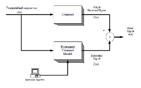
Fig. 1. Channel Estimation
The pilot based channel estimation is of two types. They are the block type and the comb type. In the block type, all subcarriers in the frame are pilot tones. Also, the frames are transmitted period- ically. In the case of comb type, only some of the subcarriers in the frame are pilot tones. Blind methods on the other hand require no training sequences. They utilize certain underlying mathematical information about the kind of data being transmitted. These methods might be bandwidth efficient but still have their own drawbacks. They are notoriously slow to converge. Their other drawback is that these methods are extremely computationally intensive and hence are impractical to implement in real-time systems. One algorithm that works for a particular system may not work with another due to the fact they send different types of information over the channel.

2.2 Kalman Filter

The Kalman filter, also known as linear quadratic estimation (LQE), is an algorithm that uses a series of measurements ob- served over time, containing noise (random variations) and other inaccuracies, and produces estimates of unknown variables that tend to be more precise than those based on a single measurement alone. More formally, the Kalman filter operates recursively on streams of noisy input data to produce a statistically opti- mal estimate of the underlying system state.
The Kalman filter estimates a process by using a form of feed- back control: the filter estimates the process state at some time and then obtains feedback in the form of (noisy) measurements. As such, the equations for the Kalman filter fall into two groups: time update equations and measurement update equations. The time update equations are responsible for projecting forward (in
time) the current state and error covariance estimates to obtain the a priori estimates for the next time step. The measurement update equations are responsible for the feedback. That is for incorporat- ing a new measurement into the a priori estimate to obtain an improved a posteriori estimate. The time update equations can also be thought of as predictor equations, while the measurement update equations can be thought of as corrector equations. Indeed the final estimation algorithm resembles that of a predictor- corrector algorithm for solving numerical problems.

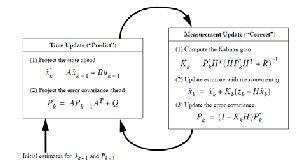
Fig. 2. Kalman Filter Prediction Estimation Cycle
The algorithm works in a two-step process. In the prediction step, the Kalman filter produces estimates of the current state variables, along with their uncertainties. Once the outcome of the next measurement (necessarily corrupted with some amount of error, including random noise) is observed, these estimates are updated using a weighted average, with more weight being given to estimates with higher certainty.

2.3 Extended Kalman Filter

The Kalman Filter algorithm was originally developed for systems assumed to be represented with a linear state-space model. How- ever, in many applications the system model is nonlinear. Fur- thermore the linear model is just a special case of a nonlinear model. Therefore, it is decided to present the Kalman Filter for nonlinear models. This technique is mainly known as an Extend- ed Kalman filter, which is a clear extension of the Kalman filtering based estimation procedure. Extended Kalman Filter (EKF) uses non-linear models of both the process and observation models while the Kalman Filter (KF) uses linear models.

International Journal of Scientific & Engineering Research, Volume 4, Issue 9, September-2013 623

ISSN 2229-5518

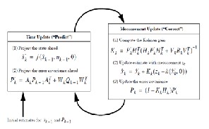
Fig. 3. Extended Kalman Filter Prediction Estimation Cycle
Figure 3 shows the Extended Kalman Filter Prediction Estima- tion Cycle which gives equations to do the estimation procedure. The Extended Kalman ﬁlter (EKF) gives an approximation of the optimal estimate. The non-linearities of the systems’s dynamics are approximated by a linearized version of the non-linear system model around the last state estimate. For this approximation to be valid, this linearization should be a good approximation of the non-linear model in the entire uncertainty domain associated with the state estimate.

2.4 Total Harmonic Distortion

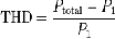
For a sine wave, the total harmonic distortion is defined as the ratio of the sum of the powers of all harmonic components to the power of the fundamental frequency. THD is used to characterize the linearity of audio systems and the power quality of electric power systems. When the input is a pure sine wave, the meas- urement is most commonly the ratio of the sum of the powers of all higher harmonic frequencies to the power at the first harmonic, or fundamental frequency. THD is also commonly defined as an amplitude ratio rather than a power ratio, resulting in a definition of THD which is the square root of that given above. The total harmonic distortion, or THD, of a signal is a measurement of the harmonic distortion present and is defined as the ratio of the sum of the powers of all harmonic components to the power of the fundamental frequency.
THD=harmonic power / signal power (2)
Lesser THD allows the components in a loudspeaker, amplifier or microphone or other equipment to produce a more accurate reproduction by reducing harmonics added by electronics and audio media. A THD rating < 1% is considered to be inhigh- fidelity and inaudible to the human ear. For household purposes, THD is below 3%. If fading is there, it is below 15%.
THD is calculated by the equation

(3)

which can equivalently be written as below if there is no source of power other than the signal and its harmonics.
superposition of multiple copies of the transmitted signal, each traversing a different path. Each signal copy will experience dif- ferences in attenuation, delay and phase shift while travelling from the source to the receiver. This can result in either construc- tive or destructive interference, amplifying or attenuating the signal power seen at the receiver. Strong destructive interference is frequently referred to as a deep fade and may result in tempo- rary failure of communication due to a severe drop in the chan- nel signal-to-noise ratio.
Rayleigh fading is the most important type of fading that oc- curs in the urban environments. It is a statistical model for the effect of a propagation environment on a radio signal, such as that used by wireless devices. Rayleigh fading models assume that the magnitude of a signal that has passed through such a transmission medium (also called a communication channel) will vary randomly, or fade, according to a Rayleigh distribution.

Fig. 4. Rayleigh probability density distributin function (pdf)
An important theorem considered in Rayleigh fading is the central limit theorem. It holds that, if there is sufficiently much scatter, the channel impulse response will be well-modelled as a Gaussian process irrespective of the distribution of the individ- ual components. If there is no dominant component to the scatter, then such a process will have zero mean and phase evenly dis- tributed between 0 and 2π radians. The envelope of the channel response will therefore be Rayleigh distributed. Rayleigh fading is a small-scale effect. There will be bulk properties of the environ- ment such as path loss and shadowing upon which the fading is superimposed.

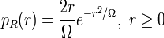
Calling the random variable R, it will have a probability densi- ty function is as given in the equation below.

2.5 Rayleigh Fading

(4)
Where

(5)
Fading is the deviation of the attenuation affecting a signal over
certain propagation media. In wireless systems, fading may either be due to multipath propagation, referred to as multipath induced fading, or due to shadowing from obstacles affecting the wave propagation, sometimes referred to as shadow fading.

3 PROJECT METHODOLOGY

(6)
The presence of reflectors in the environment surrounding a
transmitter and receiver create multiple paths that a transmitted signal can traverse. As a result, the receiver sees the
An Extended Kalman Filter is used for channel estimation. It is an extension of Kalman filter. The transmitted signal is a sine wave. We do the experiments in the presence and absence of fading. For

International Journal of Scientific & Engineering Research, Volume 4, Issue 9, September-2013 624

ISSN 2229-5518

fading, a Rayleigh fading channel is considered. The predicted estimates and updated estimates are found for both the cases. The total harmonic distortion between the updated estimate / estimat- ed state is also calculated. These are repeated for fadingless and fading channels.

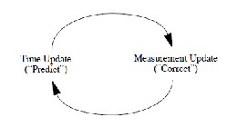
Fig. 5. Process Cycle

3.1 Flowchart

Fig. 6. Flowchart
Two stages have to be considered since we assume fadingless and fading channels for the process. The flowchart includes the vari- ous stages of the Extended Kalman filter channel estimation used in the project done. The first stage is the assumption of a commu-
nication channel for the transmission. A Rayleigh fading channel or a fadingless channel is considered. Then the initial parameters for the estimation are assumed so that the prediction and up- dation in estimation can be started. The estimation process is started and the updated and predicted estimates are found out. The errors and the total harmonic distortion are calculated then.
The THD for normal house hold purposes is less than 3% for fadingless channels. So when THD becomes within the 3% value, then the iteration is automatically stopped and the graphs are plotted for fadingless case. For the Rayleigh fading channel, a bit larger value needs to be assumed for the distortion. So in that case, 15% fading value is considered as the limit for stopping the iteration.

3.2 Algorithm

1. Start
2. Assume two channels, a fadingless channel and a Ray-
leigh fading channel.
3. Initialize the following parameters: number of iterations
(N), state error (W), measurement error (V), measure- ment state (H), process noise covariance (Q), measure- ment noise covariance (R), updated estimates, predicted estimates, actual state (x), Kalman gain (K).
4. Calculate updated and predicted states and error covari-
ance estimates, the actual state and Kalman gain for N it- erations using the EKF equations.
5. Find the errors, error1 and error2 as the difference of updated and predicted state with the actual state using the equations given below.
error1 = actual state – predicted state error2 = actual state – updated state
6. Find the total harmonic distortion (THD) of the updated sine output as the ratio of sum of harmonic powers to the fundamental power.
7. If THD >= 0.03 for the fadingless channel or THD >= 0.15 for the Rayleigh fading channel, go to step 4. Else go to step 8.
8. Plot the graphs.
9. End.
Nonlinear estimation problems are considerably more difficult than the linear problem in general. The problem with nonlinear systems is that a Gaussian input does not necessarily produce a Gaussian output (unlike linear case). The EKF even though not truly ‘optimum’, has been successfully applied in many non linear systems over the decades. The fundamental assumption in EKF design is that the true state is sufficiently close to the estimated state at all time, and hence the error dynamics can be represented fairly accurately by the linearized system about.

4 RESULTS

The actual state, updated state and the predicted state have been calculated. Then the errors and the THD also are calculated. The iteration is stopped when the THD comes inside the 3% for fad- ingless case and 15% for the Rayleigh fading case.

International Journal of Scientific & Engineering Research, Volume 4, Issue 9, September-2013 625

ISSN 2229-5518

The below given are the findings.

4.1 Fadingless Channel

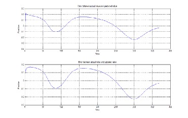
Fig. 9: The error between the predicted and updated state with the actual state.
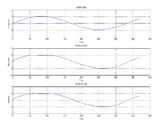
Fig. 7: The actual state, predicted state and the updated state.
The actual state is the actual sine wave which is to be received as per the equation of the EKF. The predicted state and the esti- mated/updated state are also shown in the fig. 7.

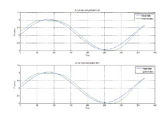
Fig. 8: The combined fig. of the actual, predicted and updated state.
The fig. 8 makes it possible to exactly find the difference pre- sent in between the actual state, predicted state and the updated state. We can see that there are distortions for the predicted and updated sine wave outputs compared to the actual wave. The actual wave is the actual state that had to be received at the re- ceiver. The distortions indicate the error or fault associated with the Extended Kalman Filtering estimation method.

The fig. 9 shows the error between the actual state and the pre- dicted state, error1 and the error between the actual state and the updated state, error2 in a large scale. From the graph, it is clear that the error of the Extended Kalman Filter estimation method is comparatively less.
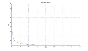
Fig. 10: The THD of the updated state.
The fig. 10 shows the total harmonic distortion of the updated state. THD is getting reduced when the number of iterations is increased. Since the code is programmed in such a way that the iteration will stop when the THD comes within 3%, the graph stops at the 368th iteration.

International Journal of Scientific & Engineering Research, Volume 4, Issue 9, September-2013 626

ISSN 2229-5518

4.2 Rayleigh Fading Channel

Fig. 11: The actual state, predicted state and the updated state.

The actual state is the actual sine wave which is to be received as per the equation of the EKF. The predicted state and the esti- mated/updated state are also shown in the fig. 11.
Fig. 12: The combined fig. of the actual, predicted and updated state.
The fig. 12 makes it possible to exactly find the difference pre- sent in between the actual state, predicted state and the updated state. We can see that there are distortions for the predicted and updated sine wave outputs compared to the actual wave. The actual wave is the actual state that had to be received at the re- ceiver. The distortions indicate the error or fault associated with the Extended Kalman Filtering estimation method.
Fig. 13: The error between the predicted and updated state with the actual state.
The fig. 13 shows the error between the actual state and the predicted state, error1 and the error between the actual state and the updated state, error2 in a large scale. From the graph, it is clear that the error of the Extended Kalman Filter estimation method is comparatively less.

Fig. 14. The THD of the updated state.
The fig. 14 shows the total harmonic distortion of the updated state. Here also, the THD is getting reduced when the number of iterations is increased. Since the code is programmed in such a way that the iteration will stop when the THD comes within 15%, the graph stops at the 464th iteration. This may change according to the initial values assumed in the iteration process.

International Journal of Scientific & Engineering Research, Volume 4, Issue 9, September-2013 627

ISSN 2229-5518

5 CONCLUSION

The Extended Kalman Filter is a set of mathematical equations that provides an efficient computational (recursive) solution of the least-squares method. The filter is very powerful in several aspects: it supports estimations of past, present, and even future states, and it can do so even when the precise nature of the mod- eled system is unknown.
There are many disadvantages for the EKF. Unlike its linear counterpart, the extended Kalman filter in general is not an opti- mal estimator (of course it is optimal if the measurement and the state transition model are both linear, as in that case the extended Kalman filter is identical to the regular one). In addition, if the initial estimate of the state is wrong, or if the process is modeled incorrectly, the filter may quickly diverge, owing to its lineariza- tion. Another problem with the extended Kalman filter is that the estimated covariance matrix tends to underestimate the true co- variance matrix and therefore risks becoming inconsistent in the statistical sense without the addition of stabilizing noise. Having stated this, the extended Kalman filter can give reasonable per- formance, and is arguably the standard used in navigation sys- tems and GPS.
The EKF has been implemented and have calculated the distor- tion of the updated estimate sine wave. This has been done in a fadingless and a Rayleigh fading environment. The distortion value has been limited below the required percentage by perform- ing different number of iterations. The reason why I used the ex- tended Kalman filter is that the system is nonlinear. So, whenever the system is nonlinear we have to use the extended Kalman filter. Of course we can also linearize the system around an operating point. But the extended Kalman filter has a better convergence than the Kalman filter, and is independent of choice of an opera- tion point.
In our case, the total harmonic distortion converged below 3%
at the 368th iteration of the estimation process as per the assumed initial values considered in this process for the fadingless system. But when we considered the fading environment, we consider the limit for the total harmonic distortion as 15% and it converged below 15% at the 464th iteration. So we can see that the iterations needed for convergence in the fading contained environment is more compared wit the fadingless environment.
The applications of the Extended Kalman filter includes track-
ing a moving object (estimate its location and velocity at each time), assuming that velocity at current time is velocity at previ- ous time plus Gaussian noise). This is done by using a sequence of location observations coming in sequentially. Future modifica- tions are possible for varying the input wave from sine wave to other square wave, triangular wave etc. Also a Modified Extend- ed Kalman Filter can be used to get a better performance. This technique has a wide range of applications in medical fields such as ECG denoising. In this medical area, future works include in- corporating baseline ﬂuctuations in the EDM to reduce the distor- tions and cause the algorithm to be more reliable. In addition, different dynamical models may be proposed to represent the new state variables behavior. Also other types of fading channels
and combined fading channels can be used. We can add different types of modulation techniques and cryptographic methods to ensure the safety of the transmitted data.

ACKNOWLEDGMENT

The platform for the work was provided by VSSC, Thiruvan- anthapuram. The authors would like to acknowledge the ref- erees for their helpful comments.

REFERENCES

[1] Rachel Kleinbauer, “Kalman filtering implementation with MATLAB”, University at Stuttgart.

[2] Gabriel Terejanu, Extended Kalman, Department of Computer Science

& Engineering, University at Buffalo, NY 14260.

[3] Rupul Safaya, "A Multipath Channel Estimation Algorithm using a

Kalman filter".

[4] Steven M. Kay, Fundamentals of Statistical Signal Processing, Volume I: Estimation Theory (v. 1).

[5] T.S. Rappaport, Wireless Communications Principles and Practice..

Publisher: Prentice Hall press. 1996.

[6] Mohinder S. Grewal, Angus P. Andrews, Kalman Filtering, Theory and

Practice Using MATLAB, Second Edition,.

[7] Vincent Poor, An Introduction to Signal Detection and Estimation.

[8] Ms. Ruchi Dahiya, Mrs. Meenu Manchanda, Mr. Manjeet, “Measuring of channel cofficient using KALMAN filter”, International Journal of Computer Science & Management Studies, Vol. 11, Issue 01, May

2011, ISSN (Online): 2231 –5268.

[9] Greg Welch & Gary Bishop, "An Introduction to Kalman Filter" , TR 95-

041,Department of Computer Science, University of North Carolina,

Chapel Hill, Chapel Hill-NC-27599-3175, 24 July, 2006.

[10] MATLAB code (m-files) for the Kalman Filtering Theory and Practice

Using MATLAB book.

[11] Deepmala Singh Parihar , Prof. Ravi Mohan, “Channel Estimation in Multipath fading Environment using Combined Equalizer and Diversity Techniques”, International Journal of Scientific & Engineering Research Volume3, Issue 1, January 2012 1 ISSN 2229-5518.