Inte rnatio nal Jo urnal o f Sc ie ntific & Eng inee ring Re se arc h, Vo lume 3, Issue 2, February -2012 1

ISS N 2229-5518

Exact solution of a problem of dynamic

deformation and nonlinear stability of a problem with a Blatz-Ko material

Edouard DIOUF

Abs tract - The aim of the paper is to study the phenomena of stability of a hollow tube subjected to combined def ormations. The model used is that of Blatz-Ko in compressible and dynamic. Bef ore studying the stability, w e have solved a boundary value problem w ith exact solution. The results could be applied in bio mechanics.

Ke ywords -systems of nonlinear equation, exact solution in dynamic, strength theory of Blatz-Ko material, stability theory of structure

——————————  ——————————

1. INTRODUCTION

For the mathematical description of many mechanical or physical pr oblems, it is often necessary to solve equations or systems of differ ential equations, to sear ch for per iodic or stationary solutions to study their stability properties. The fir st r esults of the stability theor y of nonlinear equations with Lyapunov appear ed in the late 19 th century and ear ly 20th century . He then gives a sufficient condition for stability of nonlinear systems. Chataev, meanwhile, will show a theor em of instability. Massera demonstrates a necessary and sufficient condition for stability. Hahn and Lefschetz will contr ibute to this theory [1]
Subsequently, many theor ies on stability have been
developed.
The first step in the qualitative theory of autonomous differ ential equations is an analysis of fixed points and their stability. This leads on naturally to a study of how the behavior near such fixed points can change as a parameter
is varied [2].
Ther e may be some parameter s for w hich the system
behavior changes fr om one qualitative state to another (the attractor of the system was a state of equilibr ium and becomes a cycle for example [ 3,4,5].
In this w or k, w e use non-autonomous differ ential equations. Initially, w e ar e concerned w ith axisymmetr ic finite axial shear deformation of an isotr opic compr essible dynamic nonlinear elastic hollow cir cular cylinder .
Studies on the stability of such structur es have been developed. For example the buckling and postbuckling of
cylindr ical shells under combined loading of exter nal pr essur e and axial compr ession ar e demonstr ated [6]. The
instability analysis of a cir cular and thick cylinder under hydr ostatic pr essur e is also studied [ 7].
The stabilization of the functionally graded cylindrical shell
under axial harmonic loading is investigated by Ng and al. [8]. The authors such as Roxbur gh and Ogden [ 9], Vandyke and Wineman [10] studied the vibr ations and stability of finite deformed compr essible mater ials.
The aim of this paper is firstly looking for an exact solution of the pr oblem of r adial deformation and axial shear and also the study of the stability of the solution.
For finding the exact solution, the purpose of the pr esent paper is to further examine this issue for compr essible materials as the solid Blatz-Ko mater ial. We r estrict the domain geometry to be that of a circular cylinder .
For a cir cular cylinder composed of an arbitr ary isotr opic
incompr essible elastic material, an exact solution to the
axial shear pr oblem given rise to axisymmetr ic anti-plane shear deformation has been obtained by Adkins [11].
Less than in the case of incompr essible materials, exact
solutions w er e obtained for compr essible mater ials in the static case such as the finite torsion and shear ing of a compr essible and anisotr opic tube [ 12] or dynamic as is the case, for example of the finite azimuthal shear motions of a transver sely isotr opic compr essible elastic and pr estr essed tube [13]. To study stability, w e use the technique of perturbation [14]. The question one might ask is w hether w e per turb a system of differ ential equations, the solutions obtained do they change much?
If the solutions of the perturbed system ar e all close to the

Edoua rd DIOUF, Dé parte ment de Ma théma tiques , Univers ité de Ziguinchor, BP 523 Ziguinchor Séné ga l

I nterna tiona l Journa l of Scie ntific & Enginee ring Re search Volume 3, Iss ue 2, Februa ry 2012 2

ISSN 2229-5518

solutions of the system star ting, w e talk about stability.

r (R, t) 0 0 

 

When some disturbances cr eate new solutions, instead of

F   0



r (R, t)

0 ,



(2.4)
starting solutions, w e w ill talk of instability. W e've taken
the advantage of not giving a gener al definition of stability

 h(R, t

0  

for nonlinear differ ential equations, in or der to allow the concept of stability its multifaceted character .

The Cauchy -Gr een tensors C  F T F and B  FF T ar e given by

2. Formulation

 r (R, t)2



2 r(R, t) 2

r (R, t).h(R, t )



B   0



r(R, t)   

R 2

0 ,



Rubber or other polymer mater ials ar e said to be
hyper elastic [15]. Usually, these kind of marter ials under go lar ge deformations. In or der to descr ibe the geometr ical transfor mation pr oblems, the deformation gradient tensor
is intr oduced by

r (R, t).h(R, t)

(2.5)

r (R, t )2  h(R, t )2

0 2  h(R, t)2 

0 h(R, t)

F  I  grad ( u),

(2.1)



C   0



r(R, t)2

R 2



0 ,



(2.6)
wher e I is the unity tensor and u the displacement vector. Because of lar ge displacements, Gr een-Lagrangian strain is adopted for the nonlinear r elationships betw een strains and

 h(R, t )

0 2 

displacements [15]. W e note the r ight and left Cauchy -
Gr een deformation tensor r espectively by C  F T F and B  FF T . The Gr een-Lagrangian strain tensor E is defined by

wher e X   X / R.

In the case of hyper elastic law , ther e exists a strain ener gy
density functionW which is a scale function of one of the strain tensor s, whose der ivative with r espect to a str ain component determines the corr esponding str ess

E  (C  I ) / 2,

(2.2)
component. This be expr essed by the second Piola-Kir choff str ess tensor
W e ar e concerned w ith axisymmetr ic finite radial
deformation and axial shear of an isotr opic compr essible nonlinear elastic hollow circular cylinder . Thus the deformation, which takes the point w ith cylindr ical polar

S  W

E

(2.7)

coor dinates R, , Z  in the undefor med r egion to the

point r, , z  in the deformed r egion, has the form

This gives in the cas of isotr opic hyper elasticity [16]

S  2 W

 W

 2  I

 W



C  I 3

W 

C 1  (2.8)

r  r(R, t),

  ,

z  Z  h(R, t)

(2.3)

C  I1 1 I 2 

I 2

I 3 

Wher e r(R, t)

and h(R, t)

ar e unknown functions to
wher e

tr( ),

tr(

)2

tr

2 / 2,

det( ),

determine and r epr esent r espectively the radial

I1 

C I 2 

C  C

I 3  J  C

deformation and axial shear .
With r espect to the cylindrical polar coor dinates system, the physical components of the deformation gr adient tensor is given by
denote the invariants ofC and B.
In this study, w e use a Blatz-Ko material. For a solid Blatz - Ko material, under going a deformation character ized by a deformation gr adient F , the str ain-ener gy functionW is
given by [17]

I nterna tiona l Journa l of Scie ntific & Enginee ring Re search Volume 3, Iss ue 2, Februa ry 2012 3

ISSN 2229-5518

  r R t

r  R t 

W   I

2 1

 3   I 1 /  1,

(2.9)
 r r

  R



( , )



( , ) 

,

 r (R, t ) r (R, t ) r (R, t )2 

wher e  and  ar e constants.

 2 R r (R, t )

     R r (R, t )  r (R, t ) ,

The blatz-Ko models for polyur ethane rubber have been
extensively used to descr ibe the behavior of compr essible



 R



 2  r (R, t ) r (R, t ) 

 ,

(2.15)

 z z    R 

hyper elastic isotr opic mater ial under going deformati on [18].
By der iving the ener gy density (2.9 ) with r espect to the thr ee

 r (R, t ) r (R, t )  h(R, t )2 

 R h(R, t )

invariants I1 , I 2 , I 3 , and r eporting the r esult in (2.8), w e obtain

 r z

 , 

 r (R, t ) r 

   z

 0.

S  2 J C 1  1 I

(2.10)
The motion equations in the absence of body for ces ar e

 

 

div(σ)  a 0 / J ,

(2.16)
Taking into account the kinematics (2.3) and definitions of
the invar iants of C, we get:
wher e a is the acceleration and  0 the mass density in the
r efer ence state. Equations (2.16), for the deformation (2.3),

tr( )

2  (

, )2

 ( , ) r(R, t) ,

I1 

B  

 r  R t

 h R t 2 

R 2

r educe to the following two equations:

I  det(B)  J 2 

2 r(R, t)2 r (R, t)2

R 2

(2.11)
The Cauchy str ess tensor σ is calculated fr om the second
Piola-Kir choff str ess tensor S as follows:

R 2 r  (R, t)  R r (R, t)  r(R, t)   0 R 2  r(R, t)  0,

(2.17.a)

σ  1 FSF T

(2.12)
 t 2
 2

R h (R, t)  h(R, t) 

0 R  h(R, t)  0.

(2.17.b)
which allows for taking into (2.9) and (2.10), as follows fr om
 t 2

σ

σ   0 1  1B,

(2.13)

To solve the system (2.17), w e pr opose forms of r(R, t)

and h(R, t) below [12, 13]

The elastic r esponse functions  s   s (I1 , I 3 ), (s  0,1) ar e given

r(R, t)  f1 (R) cos(wt)  f 2 (R),

h(R, t)  h (R) cos(wt)  h (R).

(2.18)

1 2

by [19]
 0  2J

I 3W3 ,

1

(2.14)

wher e f1 (R), f 2 (R), h1 (R) and h2 (R) ar e unknowns functions to

determine.
1  2J

W1 ,

Substituting equations (2.18) in those of (2.17), w e obtain a

wher eWi  W / I i , (i  1,3), and we set   2 in (2.9).

system of four equations decoupled

f  R

1 f  R



 m 2

1  f R

(2.19.a)
Substituting (2.5), (2.9) and (2.14) in (2.13), w e obtain the
components of Cauchy str es s tensor

( ) 

1 R

1 ( )  



 (

R 2  1

)  0,

I nterna tiona l Journa l of Scie ntific & Enginee ring Re search Volume 3, Iss ue 2, Februa ry 2012 4

ISSN 2229-5518

f  (R)  1 f (R)  1

f (R)  0,

(2.19.b)

wher e (n)  (n)

[21] is the logarithmic der ivative of the

2 R 2

R 2 2

(n)

gamma function.

h (R)  1 h(R)  m2 h (R)  0,

(2.19.c)

1 R 1 1

The solution of the equation (2.19.b ) is given by

h (R)  1 h (R)  0.

(2.19.d)

2 R 2

f (R)   R  1 ,

(3.3)
wher e m 2   w2 / .

2 0 R

The boundary conditions ar e
The solutions of equations (2.19.c) and (2.19.d) ar e
r espectively

r (Ri ,0)  Ri ,

r (Ro ,0)  Ro ,

h1 (R)  0 J 0 (m R),

(3.4)

h(Ri ,0)  0,

h(Ro ,0)  0,

(2.20)

h2 (R)   R

 1 ,

(3.5)

 rr (Ro , t )  0.



Wher e J 0 ( x)  

k 0

( x 2 / 4)k

k!(1  k )! , and 0 ,  , 0 , 1
ar e constants of
wher e Ri and Ro denote the inner and outer radii in the
undeformed configuration.
integr ation determined fr om the boundar y conditions (2.20).

J1 (x) and J 0 (x)

ar e ser ies of functions of the form n0 f n ( x) ,

2 n1

 

3. Resolution

Seeking the exact solutions of nonlinear partial differ ential
wher e

f n ( x)

  x 

 2 

(1)

k!(1  k )!

ar e defined on the same
equation play an important role in the nonlinear pr oblems [20]. This is the case of Bessel type equations encounter ed in many mechanical pr oblems, particular ly those w ith cylindr ical symmetry.

interval I  [Ri , Ro ]. The ser ies n0 f n ( x) conver ges normally

on the interval I [22].
Equation (2.19.a) is a Bessel equation whose solution is:

Mor eover , the functions f n (x)

ar e differ entiable on I and the

 df ( x) 

is also normally conver gent

f1 (R)  0 J1 (m R)  1Y1 (m R),

(3.1)
ser ies of function 

 n 

n0  dx 

wher e  0 and 1 ar e constants of integration determined fr om
on I .
It follows that n0

f n ( x) is differ entiable on I and w e

the boundary conditions (2.15), and J1 (x), Y1 (x) of Bessel d

 df ( x) 

get  0 f ( x)  0 

 [22].

functions of first order , r espectively fir st and second kind
defined by

dx n

n  dx 

 x 

 k  x 

This is w hat gives meaning to the last equation of boundary
conditions (2.20).

J ( x)    

( 1)

  ,

1  2 

k 0

k!(1  k )! 2 

 x   x 

(3.2)
The Cauchy-Lipchitz theor em [23] applied to the system
consisting of (2.17) (2.19) and (2.20) ensur es the existence and

Y ( x)  2 J ( x)Log

  1

2  (1) .

1  1

 2 

  x 

uniqueness of solutions (3.1) (3.3) (3.4) and (3.5).

Thus, the deformation defined in (2.3) for (R,t)  I  0,, is

given by:

I nterna tiona l Journa l of Scie ntific & Enginee ring Re search Volume 3, Iss ue 2, Februa ry 2012 5

ISSN 2229-5518

r (R, t )   J (mR)   Y (mR)cos(w t)   R  1 ,

the Cauchy-Gr een tensor s B  F F

and C  F T F ,

0 1 1 1

R (3.6)

h(R, t)   J (mR) cos(w t)  1 R 2   .

and the Cauchy str ess tensor

0 0 2

σ  0 1  1 B , wher e

Using the Cauchy-Lipchitz theor em, we can define the

1 1

concept of maximal solution, i.e. solutions defined on an open interval I  O  I  0, which can not be extended to

0  2J I3W3 , 1  2J W1 , J 

I3 

det(B ).

solutions over a r ange gr eater than I  O.

The perturbed equation of motion is given by

4. Stability

div(σ )  a 0 / J ,

(4.3)
This section is devoted to the concept of stability for the equations (2.17) and their solutions. This is a first step to disrupt the equations [14] to find new solutions, r elatives or not starting solutions. This w ill serve as a basis for discussion on the stability or instability of certain solution [24, 25]. How ever , we took advantage of not giving a general definition of stability , to allow his character to this multifaceted concept .
To find the evolution of the fluctuations ar ound solutions
(3.6), we apply the techniques of disr uptions by asking
wher ea is the acceler ation due to the kinematics (4.1).

By neglecting all quadratic terms (in  n , n  2 ), in  l s , (l, s  r, , z) , the equations of motion (4.2) become of the form A   B  0,  , which gives A  0, B  0. The equations of motion (4.3) w ill then r educe to:

 R 2 r  (R, t)   Rr (R, t) 

r (R, t) r(R, t).

 2 r(R, t)  0, (4.4.a)

  r(R, t)   R 2 

~r  r(R, t)   .F (R, t),

~z  .Z  h(R, t)   .H (R, t),

(4.1)

 0

 R 2 r (R, t ) r (R, t ) F (R, t )

t 2 

   R 2 r  R t  

wher e r(R,t), h(R,t) ar e the solutions defined en (3.6),  is a  

( , )

r (R, t ) F (R, t ) 

small par ameter quantifying the magnitude of disturbance

  r (R, t )

 



 2 F (R, t )

and F (R, t), H  (R, t) ar e unknown function to determine.

  0 R r (R, t )r (R, t )

 

t 2

(4.4.b)

  r (R, t ) r (R, t )  R 2 r  (R, t ) 

W e set as a new kinematics



 2 r(R, t )

 F  0,

 R 2 r (R, t )  r (R, t )  

~r  r(R, t)   .F (R, t),

~z  .Z  h(R, t)   .H

~  , (R, t).

(4.2)

 0

t 2 

 R h (R, t)   h(R, t)

In t his new kinematics, we will note the gradient of deformation tensor

r (R, t) r(R, t) 

  R

 0

 2 h(R, t)

t 2

  0, (4.4.c)



 F R t

  R H  (R, t )   H  (R, t )

 (

 R

, )  r' (R, t ) 0 0 





  2 H



(R, t)

r (R, t )r f (R, t ) 

F   0

 

 F (R, t )  r(R, t)

0 ,



  0 R

t 2 

(4.4.d)

 H R t

  h(R, t)   R h (R, t)

( , )

   h' (R, t

0  

  r (R, t ) F(R, t) 

 R

  

 h(R, t)

 ( , )

( , )

  0.

  0 R



t 2

 r  R t F R t 

I nterna tiona l Journa l of Scie ntific & Enginee ring Re search Volume 3, Iss ue 2, Februa ry 2012 6

ISSN 2229-5518

Methods for determine of periodic solutions have been

~r  r (R, t )   f (R)   f

(R)cos(w t)

 1 2

significantly impr oved thanks lar gely to the w or k of M.

  f

(R)   f (R),

Poincar e. We can not be said, it seem, mor e general

~z  z (R, t)  Z  h (R)   h (R)cos(wt )

(4.8)
tr igonometr ic solutions. Ther e is no universal method to find

 1 2

 h (R)   h (R).

2 1

such solutions. We must ther efor e r esolve to r estr ict our field
of study. Thus in this section, on the hand w e want to pr ove

the existence of a solution and also gener alize the r esults obtained in (3.6). Ther efor e as an example of r esolution , w e pr opose for the functions F (R,t) and H (R, t) of the following:

F (R, t)  F 1 (R) cos(wt)  F 2 (R),

5. Discussion

We pr opose in this paragr aph, to discuss the r adial deformation. Pr ovided that the same discussion and the same r emar ks can be applied to axial shear .

  

(4.5)
Periodic solutions (3.6) and (4.8) ar e time-dependent. For

H (R, t)  H 1 (R) cos(wt)  H 2 (R).

  

wher e F1 (R), F 2 (R), H 1 (R) and H 2 (R) ar e unknowns functions

   

to determine
It follows the system of equations
time per iodic solutions, ther e is a minimum time interval

T  0 (the per iod) after which the system r eturns to its or iginal state.

The solution r (R, t) as defined in (4.8) is a continuous funct ion in (R, t) . The conver gence of the ser ies J1 (mR) , Y1 (mR) and J O (mR) can show that the function r (R, t) is L -Lipchitz in the var iable R : ther e exists a

constant L such that:

d 2 F 2 (R

) 1 dF 2 (R

 

)   m2 

1  2

F (R)  0,

(4.6.a)

r (R , t)  r (R , t)  L R

 R ,  R , R  R , R . , (5.1)

dR 2

2 1

R dR 

R 2    a

 b a b

a b i o

d F (R)  1 dF (R)  1

F 1 (R)  0,

(4.6.b)

The fact that r (R, t)

is L -Lipchitz, gives a condition of

dR 2

2 2

R dR

R 2 



stability or instability w ith r espect to perturbation. W e can find a constant L0 as

d H (R)  1 dH (R)  m2 H 2 (R)  0,

(4.6.c)

dR2 R dR

 r (R, t)  r(R, t)  

f (R) cos(w t)  f (R)  L

 2

,  R  R , R , t  0.

(5.2)

i o

2 1 1

d H (R)  1 dH (R)  0.

(4.6.d)

dR 2

R dR

This inequality and the Cauchy-Lipchitz theor em [ 26, 27] show that the boundary pr oblem (4.6 ) is w ell posed; ensur e the uniqueness of the solution. In general, w e can say that a solution to a pr ob lem is stable if it is insensitive to variations
Equations (4.6.a), (4.6.b), (4.6.c) and (4.6.d) corr espond to
equations (2.19.a), (2.19.b), (2.19.c) and (2.19. d), r espectively . We deduce then the solutions (4.6):

F 2 (R)  f (R),

F 1 (R)  f (R),

in data. W e can inter pr et the sensitivity of the solution by the constant L0 .
This sensitivity allows us to discuss the phenomena of stability. W e will say that ther e ar e phenomena of instability when the constant L0 is high and stability w hen it is small.

H 2 (R)  h (R),

H 1 (R)  h (R).

(4.7)
Note that when  tends to zer o, the solution (4.8) tends to the
solution (3.6), i.e.to a lack of disturbance.
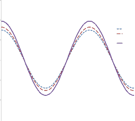
For the simulation, w e use the numerical values of the hollow
The solution of the perturbed problem , taking account of (4.1)
and (4.7) is given by

cylindr ical tube: Ri  3mm, R0  3,5mm; and w  2

[13].
In the following figur e, w e pr esent the sensitivity of the solution to perturbations.

I nterna tiona l Journa l of Scie ntific & Enginee ring Re search Volume 3, Iss ue 2, Februa ry 2012 7

ISSN 2229-5518

3,30E-03

3,10E-03

2,90E-03

2,70E-03

2,50E-03

2,30E-03

2,10E-03

ε=0

ε=0,001 ε=0,002 ε=0,003

0 0,25 0,5 0,75 1 1,25 1,5

Influe nce o f pe rturbatio n o n the radial de fo rmatio n r (Ri , t) (m) v s. time (s)

[1] W . Hahn, Theory and Application of liapunov’s Direct

Method. Pr entice-Hall inc., 1963.N.J.

[2] P.A.Glendinning, Stability, instability and chaos: an introduction to the theory of nonlinear

differential equations, Cambr idge Texts in Applied

Mathematics, CUP 1994.
[3] J.K.Hale, Asymptotic Behavior of Dissipative Systems,
Pr ovidence: Math. Surveys and
Monogr aphs, Amer . Math.Soc.1988.
[4] R. Temam. Infinite-Dimens ional Dynamical Systems in

Mechanics and Physics, Spr inger-Ver lag, New-Yor k

1988 (1st edition) and 1996 (2nd edition).
[5] D.Henry, Geometric theory of Semilinear Parabolic

Equation, Spr inger Lectur e Notes in

Mathematics, Vol.840, Spr inger Verlag, Ber lin 1984.
[6] H.S.Shen, T.Y.Chen, Buckling and postbuckling behavior

of cylindrical shells under co mbined

pressure and axial compress ion, Thin-Walled Str uct. 12

Constant sensitivity L0 as defined in (5.2) can be estimated by
(1991) 321-334.
[7] M.Bar ush,J.Singer , Effet of eccentricity of stiffners on the
L0



  



sup



 f (R) 



f (R)   (0,13).

2 

general instability of stiffened

cylindrical shells under hydrostatic pressure, J. Mech. Eng.

R  Ri , Ro  

In view of the value of L0 , w e can estimate a r elatively low instability of the solution (3.6).
Note that the stability constant is pr oportional to disturbance. But it should be noted is that this constant is independent of time.
We answer ed questions about the w ell posedness of boundary value pr oblems. Note that the magnitude of R incr eases with the disturbance. W e also note that even it is r elatively small; the disturbance is a significant influence on the system.
As an application of this study, w e think of a str uctur e or pr ototype arter ial disturbed by a disease such as an ather oscler otic plaque.

How ever , we noted that the stability constant is not informative to understand what happens over long times. It should also be noted that in this appr oach, all quadr atic terms in  , ( n , n  2) ar e neglected.

REFERENCES
Sci. 5 (1963) 23-27.
[8] T.Y.Ng, Y.K.Lam, K.M.liew , J.N.Reddy, Dynamic stability analysis of functionally grated

Cylindrical shells under periodic axial loading, Int.J. Solids

Struct. 38 (2001) 1295-1300.
[9] D. G. Roxbur gh and R. W. Ogden. Stability and vibration of pre - stressed co mpressible elastic

plates. Inter national Jour nal of Engineer ing Science,

32(3):427-454, 1994.

[10] T.J.Vandyke,A.S.Wineman, Small amplitude s inusoidal disturbances supe rimposed on finite

circular shear of a compressible, non-linearly elastic mate rial, Int. J. Ing. Sci.,34 (1996)

1197-1210
[11] J.E.Adkins, Some generalizations of the shear problem for isotropic incompressible mate rials,
Pr oc. Cambr idg Philos. Soc. 50, 334 -345 (1954).
[12] M.Zidi,Finite torsion and shearing of a compressible and

anisotropic tube, Int. Journal of

Non linear Mechanics, 35:1115 -1126 (2000).
[13] E.Diouf,M.Zidi, Finite azimuthal shear motions of a transversely isotropic co mpressible elastic

And pretressed tube, Int. J. Ing. Sci., 43 :262-274 (2005). [14] Jouve F.,Modélisation de l’oeil en élasticité non linèaire, Masson, Paris, 1993.

I nterna tiona l Journa l of Scie ntific & Enginee ring Re search Volume 3, Iss ue 2, Februa ry 2012 8

ISSN 2229-5518

[15] Zhi-Qiang Feng, B. Magnain, J. Cros, Solution of large deformation impact problems with

friction between Blatz-Ko hyperelastic bodies. Int. J. Ing. Sci. 44 (2006) 113-126.

[16] P.G. Ciarlet ,Elasticité tridimens ionnelle, Masson, Collection, RMA, 1985.
[17] M. Destrade,G.Saccomandi,On finite amplitude elastic waves propagating in compressible

solids.(2005) Physical Review E.

[18] M.Destrade,Finite-Amplitude inhomogeneous plane waves

in a deformed Blatz-Ko Materal,

CanCNSM, Victoria, June 16-20, 1999.
[19] A.D. Polignone, C.O. Hor gan, Axisymmetric finite anti-

plane shear of compressible nonlinealy

elastic circular tubes.Quarter ly of applied mathematics,

Vol.L, N.2, j une 1992, Pages 323-341.
[20] C.Tr uesdell, W .Noll, The non-linear field theories of mechanics, Handbuch der Physik, III/3
(S.Flugge, ed.), Springer-Ver lag, Berlin, 1965.
[21] F.Lar oche,Promenade Mathématiques, Fonctions de Bessel, pr omenadesmaths.fr ee.fr , 2004.
r idge University Pr ess, 1998.
[22] C. Deschamps, A. Warusfel,Mathématiques Tout-en-un.

2ième année MP,

2ième edition Dunod, 2004.
[23] A.M. Stuart, A.R.Humphries,Dynamical systems and

nume rical analysis,Cambr idge University

Pr ess, 1998.
[24] E.Hebey,Nonlinear elliptic equations of critical Sobolev growth from a dynamical viewpoint
Noncompact pr oblems at the inter-section of geometry, analysis, and topology, Contemp.
Math., vol. 350, Amer . Math.Soc., Pr ovidence, RI,
2004,p.115-125.
[25] O.Dr uet, E.Hebey, J. Vétois, Boundary stability for

strongly coupled critical elliptic systems below the geometyric threshold of the conformal Laplacien,J. Funct . Anal. 258 (2010), No.3,p. 999-1059.

[26] T.Kato, Pertubation theory for linear operator,Classic in Mathematics, Spr inger-Verlag,Berlin, 1995, Reprint of the 1980 edition.
[27] A.M.S., A.R.Humphr ies, Dynamical systems and nume rical analysis. Camb