International Journal of Scientific & Engineering Research, Volume 4, Issue 8, August-2013 1143

ISSN 2229-5518

Error minimization in Variable Fractional delay

FIR Digital Filter

Preeti Gulati, Prof. Karamjeet Singh

Abstract:-The Digital filters having changeable frequency responses are called variable digital filters. Basically, variable digital filters include those with variable magnitude response or/and VFD response. The various efficient methods have also been developed for designing both FIR VFD filters and IIR all-pass VFD filters. The simplest VFD filters are the Lagrange-type VFD filters that can be derived from the Lagrange-polynomial interpolation. Lagrange-type VFD filters are a special class of FIR VFD filters whose frequency responses at frequency are the maximally flat, so they are often called the maximally flat VFD filters. Since Lagrange-type VFD filter has a closed-form impulse response that can be expressed as a polynomial in the VFD parameter, it is easy to use. Moreover, coefficient symmetry can be developed and exploited in fast hardware implementation through coefficient transformations. However, one disadvantage of the Lagrange- type VFD filters is that the passband width is rather narrow. For wideband VFD filtering applications, efficient methods for designing wideband VFD filters using both FIR and IIR all-pass transfer functions have been developed. So far, most existing design methods obtain VFD filters by approximating the desired (ideal) VFR in the W LS sense or minimax sense. The former minimizes the total error energy (integral of squared errors) of the VFR while the latter minimizes the maximum absolute error (peak error) of the VFR. Generally speaking, there is a trade-off between the two kinds of errors, i.e., the two kinds of errors cannot be simultaneously minimized by using the existing design methods. Usually, minimizing one then increases another. In the minimax design case, So develop a biminimax method for designing even-order FIR VFD filters whose VFR peak error and VFD peak error are simultaneously suppressed. More concretely, both the two peak errors are simultaneously made nearly equi-ripple, which is referred to as bi-equiripple. The most important part of the biminimax design is to linearize the highly non-linear constraints on the VFD errors as linear ones. After the linearization, the biminimax design can be easily performed by minimizing a mixed error function that contains both the VFR peak error and VFD peak error. However, minimization is a highly nonlinear problem, So we want to try iterative method for overcome it to further reduce the maximum absolute group-delay error in the least squares design, an iterative weighting-updated technique is also proposed, which constitutes the outer loop of the overall iterative process while the iteration stated earlier makes up the inner loop.

Keyword: - Finite impulse response(FIR), Infinite-impulse-response(IIR),Variable frequency response (VFR), Weighted-least- squares(W LS),Variable fractional delay(VFD).

——————————  ——————————

1 INTRODUCTION

HE variable fractional delay (VFD) digital filters as an important class of the variable digital filters have been receiving increasingly attention in the past decade. Under tuning a controlling parameter, this kind of filters changes continuously a delay, which is a fraction of the sampling period.VFD filters have many applications in different areas of signal processing and communication, for example, time adjustment in digital receivers, speech coding and synthesis, time delay estimation and analog– digital (A/D) conversion, etc. A method for developing VFD filters is also an essential technique for the fractional linear discrete-time systems. Theoretically speaking, the design of

————————————————

I. Assistant Professor. , Electronics & Communication Dept. Chandigarh

Engineering College, Landran, Mohali, INDIA cecm.ece.pg@gmail.com

II. Professor, Electronics & Communication Dept.Baba Banda Singh Bahadar

College of Engineering & TechnologyFatehgarh Sahib,Punjab, India

variable digital filters under optimal sense is more complicated and difficult than the design of fixed delay filters, since the impulse response or the poles and zeros of the filters are some type of functions in the variable parameter (are generally assumed to be polynomial functions. Therefore, suboptimal approaches for the design of variable digital filters should be investigated for the purpose of reducing the computation complexity. For instance, the two-stage approach, i.e., designing a set of fixed-coefficient filters, and then fitting each of the coefficients as polynomials, has been proposed in the literatures. Recently, advances have been made on the design of some type of VFD filters, such as finite-impulse response (FIR) VFD filters and infinite-impulse response (IIR) all pass VFD filters. However, most of the methods employed iteration algorithm to formulate the design problem. Since large numbers of coefficients should be designed, related iteration algorithms still feature considerable computation complexity.

International Journal of Scientific & Engineering Research, Volume 4, Issue 8, August-2013 1144

ISSN 2229-5518

2 DESIGN METHOD

For the purpose of comparison and the use of the conventional LS design of VFD FIR digital filters is reviewed in this section. The desired response of a VFD FIR filter is given by
obviously, I = N�2 . In this paper, only even is used, and the
case for odd can be extended in a similar manner. Notice
that the first subfilter G0 (z) is designed to approximate e−j�N�2�w , so h(n, 0) = δ�n − (N⁄2)� . Hence,
the frequency response of can be written as
Hd (w, p) = e−j(I+p)w = e−jIw (cos(wp) − j sin(wp)) ,
w ≤ wp ; −0.5 ≤ p ≤ 0.5
N

H(ejw , p) = e−j w �1

N/2

Where is a prescribed mean group delay and is the parameter used to adjust the group delay of a filter online.
+ � � a(n, m)p2m cos(nw)

m=1 n=0

Ms N/2

The used transfer function is characterized by

H(z, p) = � hn (p)z−n

n=0

where coefficients h(n) are expressed as the polynomials of
Defining
+ j � � b(n, m)p2m−1 sin(nw)�

m=1 n=1

⎡ a(0,1) … … … … … . . , a �N , 1� … … … … … … ⎤
p by
a = ⎢�
2 �⎥
N

hn (p) = � h(n, m) pm

m=0

⎢ . a(0, Mc ) … … … . a(
⎣ 2
, Mc) ⎥
⎦

⎡ b(1,1) … … … … … . . , b �N , 1� … … … . b(1, M ) … ⎤
Hence

N M

b = ⎢�
⎢
⎣
2
N
… … . b(
2
�⎥
, Ms ) ⎥
⎦
H(z, p) = � � h(n, m) pm z−n

n=0 m=0

c(w, p) = �
N

p2 … … … p2 cos �
2

w� … … … … . p2MC … …
�

m=0

Gm (z)pm
N

… p2MC cos( w)
2
Where sub filters Gm (z) are represented by
p sin(w) … … T
⎡ ⎤

N ⎢… … p sin �N w� … . p2MS−1 sin(w) … …⎥

Gm (z) = � h(n, m) z−n , 0 ≤ m ≤ M

n=0

s(w, p) = ⎢
⎢
⎣
2
N

. … p2MS−1 sin(
2
⎥
w) ⎥
Obviously, this can be implemented by the Farrow
structure .The equation can be further represented by
Equation can be written as

H(ejw , p) = e−j 2 w [1 + aTc(w, p) + jbT s(w, p)]

∞

Hd (w, p) = e−jIw �

m=0

(−jpw)m
m!

≡ � �

m=0

(−jw)m
m!
e−jIw � pm
Where the subscript .T denotes the response operator.The conventional objective error function for designing a VFD
for sufficiently large M. After compersion, it can be found that the frequency response of Gm (z) is used inherently to

FIR filter is given by

0.5 wp

approximate �(−jw)
e−jIw � for 0 ≤ m ≤ M . Therefore, it is
e (a, b) = � � W(w) |H (w, p) − H(ejw , p)|2

reasonable to choose the coefficients of Gm (z) to be
symmetric for even and anti symmetric for odd M, and

c d

−0.5 0

International Journal of Scientific & Engineering Research, Volume 4, Issue 8, August-2013 1145

ISSN 2229-5518

0.5 wp

For LS design W(w) = 1 and by applying the technique in
ec (a, b) = � � W(w)|cos(pw)

−0.5

− j sin(pw) − 1 − aT c(w, p)
− jbTs(w, p)|2dwdp
[22], the elements inra,Qa , rb , and Qb can be represented in
closed form. In this paper K must be chosen large enough
and K = 10 is used in this paper. Oncera , Qa , rb , and Qbare
obtained, the optimal solutions in the LS sense can be
achieved by differentiating with respect to a and b ,
ec (a, b) = ec(a) + ec(b)
respectively, and then setting the results to zero as follows:
Where W(w) is a weighting function

∂ec(a, b) =
∂a

∂ec(a)
∂a
= ra + 2Qa a = 0

0.5 wp

ec(a) = � � W(w)(cos(pw) − 1 − aT c(w, p))2 dwdp
∂e (a, b)
∂e (b)

−0.5 0

c = c

∂b ∂b
= rb
+ 2Qb b = 0
Which yield

T T

ec(a) = sa + ra a + a Qa a
a = −
1 Q−1 r
2 a a
1 −1

0.5 wp

b = −
Qb rb
ec (b) = � � W(w)(sin(pw) +bT s(w, p))2 dwdp 2

−0.5 0

3. PROPOSED DESIGN METHOD

T T

ec (b) = sb + rb b + b Qb b

0.5 wp

sa = � � W(w)(cos(pw) − 1)2dwdp

−0.5 0

0.5 wp

ra = −2 � � W(w)(cos(pw) − 1)c(w, p)dwdp

−0.5 0

0.5 wp

In Section 2, the VFD FIR filter is designed such that the root-mean-square error of variable frequency response can be minimized. In this section, delay-oriented minimization is proposed so that the root-mean-square group-delay error can be minimized as much as possible while the desired variable frequency response can be preserved to a certain extent.
The desired group-delay response of a VFD FIR filter can be derived from
Qa = � � W(w)c(w, p)c T(w, p)dwdp

−0.5 0

𝜕
𝜏𝑑 (𝑤, 𝑝) = −
< 𝐻𝑑 (𝑤, 𝑝) =
𝑁

+ 𝑝 ;

0.5 wp

𝜕𝑤 2
sb = � � W(w)(sin(pw))2dwdp

−0.5 0

0.5 wp

|𝑤| ≤ 𝑤𝑝 ∶ −0.5 ≤ 𝑝 ≤ 0.5
And the actual group-delay response of the designed
system is given by
rb = 2 � � W(w) sin(pw) s(w, p)dwdp

−0.5 0

𝜏 (𝑤, 𝑝) = − 𝜕 < 𝐻(𝑒

𝐻 𝜕𝑤

𝜕

𝑗𝑤

, 𝑝)
𝑁
𝑏𝑇 𝑠(𝑤, 𝑝)

0.5 wp

=
𝜕𝑤

�− 𝑤 + tan−1
2

1 + 𝑎𝑇 𝑐(𝑤, 𝑝)�
Qb = � � W(w)s(w, p)sT (w, p)dwdp

−0.5 0

International Journal of Scientific & Engineering Research, Volume 4, Issue 8, August-2013 1146

ISSN 2229-5518

𝜏𝐻 (𝑤, 𝑝)

𝑁 �1 + 𝑎𝑇 𝑐(𝑤, 𝑝)��𝑏𝑇 𝑠𝑑 (𝑤, 𝑝) − 𝑎𝑇 𝑐𝑑 (𝑤, 𝑝)��𝑏𝑇 𝑠(𝑤, 𝑝)�
= 2 − �1 + 𝑎𝑇 𝑐(𝑤, 𝑝)�2 + �𝑏𝑇 𝑠(𝑤, 𝑝)�2

𝜕
𝑐𝑑 (𝑤, 𝑝) = 𝜕𝑤 𝑐(𝑤, 𝑝)

𝜕
𝑠𝑑 (𝑤, 𝑝) = 𝜕𝑤 𝑠(𝑤, 𝑝)
Where the coefficient vectors denoted by subscript 𝑘 are to be determined in the 𝑘 th iteration and the functions denoted by subscript 𝑘 − 1 are the results of the previous
iteration, which are defined by
𝐻𝑅,𝑘−1 (𝑤, 𝑝) = 1 + 𝑎𝑇 𝑐(𝑤, 𝑝)
𝐻𝐼,𝑘−1 (𝑤, 𝑝) = 𝑏𝑇 𝑠(𝑤, 𝑝)

2 2

The objective error function of the proposed method is given by
𝐻𝑘−1 (𝑤, 𝑝) = �𝐻𝑅,𝑘−1 (𝑤, 𝑝) + 𝐻𝐼,𝑘−1 (𝑤, 𝑝)�2
Thus, the original nonlinear problem can be converted into
an iterative quadratic problem whose error function can be formulated into

0.5

𝑤𝑝

𝑒(𝑎, 𝑏) = � � 𝑊(𝑤)|𝜏𝑑 (𝑤, 𝑝) − 𝜏𝐻 (𝑤, 𝑝)|2 𝑑𝑤𝑑𝑝

−0.5 0

0.5

𝑤𝑝

𝑇 𝑇

𝑇 𝑇 𝑇

+ 𝛼 � � 𝑊(𝑤)|𝐻𝑑 (𝑤, 𝑝)
𝑒𝑘 (𝑎𝑘 , 𝑏𝑘 ) = 𝑠𝜏 + 𝑏𝑘 𝑄𝑠 𝑏𝑘 + 𝑎𝑘 𝑄𝑐 𝑎𝑘 + 𝑟𝑠 𝑏𝑘 + 𝑟𝑐 𝑎𝑘 + 𝑎𝑘 𝑄𝐶𝑆 𝑏𝑘

𝑇 𝑇 𝑇

−0.5 0

− 𝐻(𝑒𝑗𝑤 , 𝑝)|2𝑑𝑤𝑑𝑝
+ 𝛼(𝑠𝑎 + 𝑟𝑎 𝑎𝑘 + 𝑎𝑘 𝑄𝑎 𝑎𝑘 + 𝑠𝑏 + 𝑟𝑏 𝑎𝑘
+ 𝑏𝑇 𝑄 𝑏 )
𝑒(𝑎, 𝑏) = 𝑒𝜏 (𝑎, 𝑏) + 𝛼𝑒𝑐 (𝑎, 𝑏)
Where

0.5

𝑤𝑝

𝑠𝜏 = � � 𝑊(𝑤)𝑝2 𝑑𝑤𝑑𝑝
Where 𝛼 is a relative weighting constant, 𝑒𝑐 (𝑎, 𝑏) and

−0.5 0

𝑒𝜏 (𝑎, 𝑏) is shown as

0.5

𝑤𝑝

𝐻𝑅,𝑘−1 𝑇

𝑄𝑠 = � � 𝑊(𝑤) 𝐻4 (𝑤, 𝑝) 𝑠𝑑 (𝑤, 𝑝)𝑠𝑑 (𝑤, 𝑝)𝑑𝑤𝑑𝑝
𝑒𝜏 (𝑎, 𝑏)

0.5

𝑤𝑝

−0.5

0.5

𝑤𝑝

𝑘−1

𝐻2 (𝑤, 𝑝)
= � � 𝑊(𝑤) �𝑝
𝑄𝑐 = � � 𝑊(𝑤)

𝐼,𝑘−1

𝑐 (𝑤, 𝑝)𝑐𝑇 (𝑤, 𝑝)𝑑𝑤𝑑𝑝

−0.5 0

𝑘−1

(𝑤, 𝑝) 𝑑 𝑑
�1 + 𝑎𝑇 𝑐(𝑤, 𝑝)��𝑏𝑇 𝑠𝑑 (𝑤, 𝑝) − 𝑎𝑇 𝑐𝑑 (𝑤, 𝑝)��𝑏𝑇 𝑠(𝑤, 𝑝)�

+ 2
�1 + 𝑎𝑇 𝑐(𝑤, 𝑝)�

2 �

+ �𝑏𝑇 𝑠(𝑤, 𝑝)�
𝑑𝑤𝑑𝑝

0.5

𝑤𝑝

𝐻𝑅,𝑘−1 (𝑤, 𝑝)𝑝
𝑟𝑠 = 2 � � 𝑊(𝑤)

𝐻2 (𝑤, 𝑝) 𝑠𝑑 (𝑤, 𝑝)𝑑𝑤𝑑𝑝

−0.5 0

𝑘−1

Obviously, minimization of is a highly nonlinear problem, and an iterative method is proposed in this paper to replace

0.5

𝑤𝑝

𝐻𝐼,𝑘−1 (𝑤, 𝑝)𝑝
it.
𝑟𝑐 = −2 � � 𝑊(𝑤)

2 (𝑤, 𝑝)

𝑐𝑑 (𝑤, 𝑝)𝑑𝑤𝑑𝑝
The objective error function in the 𝑘 th iteration for the proposed iterative method is represented by

−0.5

0.5

𝐻𝑘−1

𝑤𝑝 𝑊(𝑤) 𝐻𝑅,𝑘−1 (𝑤, 𝑝)𝐻𝐼,𝑘−1 (𝑤, 𝑝)

𝑄𝐶𝑆 = −2 � �
𝐻𝑘−1 (𝑤, 𝑝)

𝑒𝑘 (𝑎𝑘 , 𝑏𝑘 ) = 𝑒𝜏,𝑘 (𝑎𝑘 , 𝑏𝑘 ) + 𝛼𝑒𝑐,𝑘 (𝑎𝑘 , 𝑏𝑘 )

−0.5 0

. 𝑐𝑑 (𝑤, 𝑝)𝑠𝑇 (𝑤, 𝑝)𝑑𝑤𝑑𝑝

0.5

𝑒𝑘 (𝑎𝑘 , 𝑏𝑘 ) = � �

𝑤𝑝

𝑊(𝑤)

�(𝐻2 (𝑤, 𝑝)𝑝

𝐻4 (𝑤, 𝑝) 𝑘−1

In the 𝑘th iteration, solutions 𝑎𝑘 and 𝑏𝑘 can be obtained by
differentiating with respect to 𝑎𝑘 and 𝑏𝑘 , respectively, and

−0.5 0

𝑘−1

𝑇

+ 𝐻𝑅,𝐾−1 (𝑤, 𝑝)𝑏𝑘 𝑠𝑑 (𝑤, 𝑝)

𝑇 2

then setting the results to zero

− 𝐻𝐼,𝑘−1 (𝑤, 𝑝)𝑎𝑘 𝑐𝑑 (𝑤, 𝑝)) �𝑑𝑤𝑑𝑝 + 𝛼(𝑠𝑎

𝑇 𝑇

+ 𝑟𝑎 𝑎𝑘 + 𝑎𝑘 𝑄𝑎 𝑎𝑘 + 𝑠𝑏 + 𝑟𝑏 𝑏𝑘 + 𝑏𝑘 𝑄𝑎 𝑏𝑘 )

http://www.ijser.org

International Journal of Scientific & Engineering Research, Volume 4, Issue 8, August-2013 1147

ISSN 2229-5518

𝜕𝑒𝑘 (𝑎𝑘 , 𝑏𝑘 ) = 2𝑄 𝑎
+ 𝑟 + 𝑄
𝑏 + 𝛼𝑟
+ 2𝛼𝑄 𝑎 = 0
The iterative procedures are shown in Fig. 1 and described in detail as follows.
𝜕𝑎𝑘

𝑐 𝑘 𝑐

𝑐𝑠 𝑘 𝑎

𝑎 𝑘

𝜕𝑒𝑘 (𝑎𝑘 , 𝑏𝑘 ) = 2𝑄 𝑏
+ 𝑟 + 𝑄𝑇 𝑎
+ 𝛼𝑟
+ 2𝛼𝑄 𝑏 = 0

𝜕𝑏𝑘
Which lead to

𝑠 𝑘 𝑠

𝑐𝑠 𝑘 𝑏

𝑏 𝑘

Step 1) Given ,𝑀 ,𝑤𝑝 , and and setting iterative counter
𝑘 = 0, find the initial coefficient vectors 𝑎0 and 𝑏0.

1 −1

𝑎𝑘 = − 2 (𝑄𝑐 + 𝛼𝑄𝑎 )

(𝑟𝑐 + 𝛼𝑟𝑎 + 𝑄𝑐𝑠 𝑏𝑘 )

Step 2) Increase iterative counter 𝑘 by one and calculate

1 −1 𝑇

𝐻𝑘−1 (𝑤, 𝑝),𝐻𝑅,𝑘−1 (𝑤, 𝑝) ,𝐻𝐼,𝑘−1 (𝑤, 𝑝) ,𝑄𝑆 , 𝑄𝐶 , 𝑟𝑠 ,𝑟𝑐 and 𝑄𝐶𝑆 .

𝑏𝑘 = − 2 (𝑄𝑠 + 𝛼𝑄𝑏 )

(𝑟𝑠 + 𝛼𝑟𝑏 + 𝑄𝑐𝑠 𝑎𝑘 )

After modification

𝑎𝑘 = �2𝑄𝑐 − 2 𝑄𝐶𝑆 (𝑄𝑆 + 𝛼𝑄𝑏 )

−1

−1 𝑄𝑇 + 2𝛼𝑄 �

𝐶𝑆 𝑎

Step 3) Find coefficient vectors 𝑎𝑘 and 𝑏𝑘 .
Step 4) Check whether both relative norms 𝛽𝑎,𝑘 and𝛽𝑏 ,𝑘 are

� 𝑄𝐶𝑆 (𝑄𝑆 + 𝛼𝑄𝑏 )−1 (𝑟𝑠 + 𝛼𝑟𝑏 ) − 𝑟𝑐 − 𝛼𝑟𝑎 �

small enough by

𝛽𝑎 ,𝑘 < 𝜀𝑖𝑛𝑛

−1

𝑇 −1

𝛽𝑏 ,𝑘 < 𝜀𝑖𝑛𝑛

𝑏𝑘 = �2𝑄𝑆 − 2 𝑄𝐶𝑆 (𝑄𝑆 + 𝛼𝑄𝑎 )

𝑄𝐶𝑆 + 2𝛼𝑄𝑏 �

If the condition is satisfied, stop the process; otherwise, go

1 𝑇 (𝑄

+ 𝛼𝑄 )−1 (𝑟 + 𝛼𝑟 ) − 𝑟

− 𝛼𝑟 �

to Step 2).

�2 𝑄𝐶𝑆 𝐶

𝑎 𝑐

𝑎 𝑆 𝑏

Notice that because the related matrices, whose inverses are
to be determined are symmetric and positive definite, the technique of Cholesky factorization can be applied to solve the ill-conditioning problem.
To terminate the iterative process, the relative norms are defined by
𝛽𝑎,𝑘 =
𝛽𝑏,𝑘 =

‖𝑎𝑘 − 𝑎𝑘 − 1‖
‖𝑎𝑘 ‖

‖𝑏𝑘 − 𝑏𝑘 − 1‖
‖𝑏𝑘 ‖
When both 𝛽𝑎,𝑘 and 𝛽𝑏,𝑘 are small enough, e.g., smaller than
𝜀𝑖𝑛𝑛 , where 𝜀𝑖𝑛𝑛 is a preassigned very small positive
constant, the iterative process can stop.

International Journal of Scientific & Engineering Research, Volume 4, Issue 8, August-2013 1148

ISSN 2229-5518

and the experimental results may be show that the performance in group-delay response and the convergence
of the iterative method are satisfactory.

Initiation 𝑁 ,𝑀 ,𝑤𝑝 , 𝛼,

𝑎𝑜 ,𝑏0 ,𝜀𝑖𝑛𝑛 ,𝑘 =0

𝑘 ← 𝑘 + 1

Calculate

𝐻𝑘−1 (𝑤, 𝑝),𝐻𝑅,𝑘−1 (𝑤, 𝑝) ,𝐻𝐼,𝑘−1 (𝑤, 𝑝)

,𝑄𝑆 , 𝑄𝐶 , 𝑟𝑠 ,𝑟𝑐 and 𝑄𝐶𝑆 .

Find 𝑎𝑘 , 𝑏𝑘

𝛽𝑎 ,𝑘 < 𝜀𝑖𝑛𝑛 No

And

𝛽𝑏,𝑘 < 𝜀𝑖𝑛𝑛

Yes

Stop

5 REFERENCES

[1]. An Efficient Design of a Variable Fractional Delay

Filter Using a First-Order Differentiator

Soo-Chang Pei, Fellow, IEEE, and Chien-Cheng Tseng, Senior Member, IEEE

[2]. Hybrid Structures for Low-Complexity

Variable Fractional-Delay FIR Filters

Tian-Bo Deng, Senior Member, IEEE

[3]. Improved Methods for the Design of Variable

Fractional-Delay IIR Digital Filters

Soo-Chang Pei, Fellow, IEEE, Jong-Jy Shyu, Member, IEEE, Yun-Da

Huang, and Cheng-Han Chan, Member, IEEE

[4]. Generalized WLS Method for Designing All-Pass

Variable Fractional-Delay Digital Filters

Tian-Bo Deng, Senior Member, IEEETwo-Dimensional Farrow Structure and the Design of

Variable Fractional-Delay 2-D FIR Digital Filters

Jong-Jy Shyu, Member, IEEE, Soo-Chang Pei, Fellow, IEEE, and Yun-Da

Huang

[5]. A Simple and Efficient Design of Variable Fractional Delay FIR Filters Hui Zhao and Juebang Yu

[6]. SVD-Based Design and New Structures for Variable

Fractional-Delay Digital Filters

Tian-Bo Deng, Senior Member, IEEE, and Yuko Nakagawa

[7]. Efficient Design and Implementation of Variable

Fractional Delay Filters Using Differentiators

Chien-Cheng Tseng, Senior Member, IEEE, and Su-Ling Lee

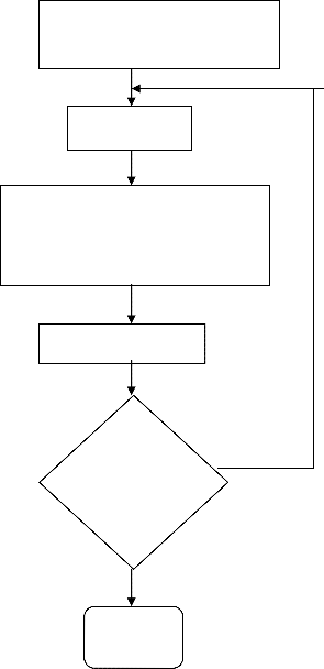
Flow Chart for proposed method

4. CONCLUSION

In this paper, a new method for the minimization of the root-mean-square error of variable group-delay response has been proposed for the design of VFD FIR digital filters. To overcome the nonlinear optimization for minimization, the proposed iterative method can be successfully used,