International Journal of Scientific & Engineering Research, Volume 4, Issue 9, September-2013 2473

ISSN 2229-5518

Eigenvalue Analysis of Microwave Oven

Hussnain Haider, Muhammad Faheem Siddique, Syed Haider Abbas, Awais Ahmed

Sarhad University of Science and Information Technology, Pakistan.

Abstract— In this research, we have used COMSOL Multiphysics to model the Microwave oven. The geometrical model of microwave oven is then used to find the resonant frequency and quality factor along with the plots for each eigenvalue. It was observed that quality factor drops with the increase in the number of hotspots. In addition, the same values and plots are obtained for a microwave with 1 liter of water load.

Index Terms— Microwave Oven, Eigenvalues, COMSOL Multiphysics, Quality factor.

——————————  ——————————

1 INTRODUCTION

he waveguides are used as a type of transmission lines, therefore resonators can also be built from closed sections of waveguide. The waveguide resonators are short circuit-
ed at both ends to prevent radiations and known as closed box or cavity. Electric and magnetic energy is stored in the cavity while power is dissipated in the metallic walls of the cavity and in dielectric filling the cavity. Coupling to the resonator is done by a small aperture or small probe. The two things which are important to derive are the equation for resonant frequen- cies (TEmnl and TMmnl ) and the quality factor.
The geometry of rectangular cavity (figure 2.1) is such that it consists of a length which is shorted at both ends (z = 0). We begin with the general TE and TM waveguide fields, which satisfy the boundary conditions on the side of walls (x =
0,a and y = 0,b) of the cavity. We know it is important to im- pose that Ex = Ey = 0 on the other end (z = 0,d). The transverse electric fields (Ex , Ey ) of the TEmn or TMmn rectangular wave- guide mode can be written as:

Et(x, y, z) = e(x, y) [A+ + A- ]

Where e(x, y) is the transverse variation of the mode, and A+, A- are amplitudes of the forward and reverse travel- ling waves. We can observe that different modes with same set of m, n, and l have the same resonant frequency irrespective of the actual field distribution. Modes with the different field patterns but having the same resonant frequency are called degenerate modes. Some other vital observations for rectangu- lar cavities are:
• Resonant frequency increases with increasing mode hav- ing fixed box size. It is possible when waves get shorter (dimension is fixed) which means that frequency will in- crease.
• The rectangular box or cavity has to be increased to ac- commodate higher modes for a given resonant frequency.
• Higher Q can be attained by going for higher modes for a given resonant frequency.
We are working on microwave oven, from our prior knowledge; we know this that they work on 2.45 GHz. On the basis of this cutoff frequency equation shown in 2.5, a pro- gram in Matlab was written to fetch out the modes that can be present in microwave. We downloaded a datasheet for Pana-
sonic MN-SD259WBPQ microwave oven (22 L) to get the di- mensions and find out the available modes. According to the specifications a = 0.33m, b = 0.325m and c = 0.218m. The cutoff frequencies in between 2.35 GHz and 2.55 GHz were given more importance and shown below in table 1.

TABLE 1

MODES BETWEEN 2.35 – 2.55 GHz

COMSOL Multiphysics uses the proven finite element method (FEM) for solving the models. The software runs the finite element analysis together with adaptive meshing and error control using a variety of numerical solvers. PDEs form the basis for the laws of science and provide the foundation for modeling a wide range of scientific and engineering phe- nomena. Therefore we can use it in many applications such as acoustics, bioscience, diffusion, electromagnetics, fluid dy- namics, heat transfer, microelectromechanical systems (MEMS), microwave engineering, optics, radio-frequency components, structural mechanics and wave propagation. Many real-world applications involve simultaneous couplings in a system. We will be using this software for out modeling and analysis.

2 STRUCTURE OF A RECTANGULAR CAVITY

The research was a commercial project from Panason- ic, which was divided into two parts; simulation through software and practical experiments on the microwave oven provided. Therefore, it was necessary for my part (simulation) to have the exact dimensions of the microwave oven given by Panasonic. In the model navigator, new file with 3D space di-

IJSER © 2013 http://www.ijser.org

International Journal of Scientific & Engineering Research, Volume 4, Issue 9, September-2013 2474

ISSN 2229-5518

mension and Electromagnetic waves from RF module was selected. The basic structure of the microwave cavity with the dimensions i.e. 35cm × 22.5cm × 27.1cm was created in the main environment
The material used for the walls of the microwave cav-
ity is Ferritic Steel S430 with conductivity 1.67×106 Siemens

per meter. The basic structure of the rectangular cavity shown in figure 1.

Figure 1, Structure of a Rectangular Cavity

2.1 Eigenvalue analysis for empty cavity

Eigenvalue analyses are obtained for the empty cavity and with 1Litre of water. This will give us a general idea of how the electromagnetic waves will be present and what will be the pattern inside the rectangular box. The meshing free parameters and the solver parameters are fetched for harmon- ic analysis with 16 eigenvalues around 2.45 GHz.
The linear system solver is set to Direct (PARDISO) which is the best linear solver when it comes to electromagnet- ic waves. The best thing about this solver is that it gives solu- tion efficiently by using less memory than other linear system solvers. All other tabs are set as default. The microwave cavity is then simulated by pressing the solve button. The successful completion of simulation will result in the plot for the last ei- genvalue. In the next stage, slice plot of electric field for each x-axis, y-axis and z-axis is plotted from postprocessing menu.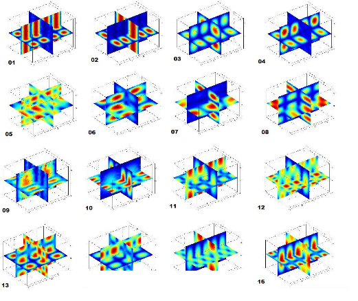

The values (Resonant frequency and Quality Factor) and plots for each eigenvalue are fetched through postpro- cessing plot parameters and global data display respectively. Plots for all the eigenvalues and values of resonant frequency plus quality factor are shown in figure 2 and table 2 respec- tively.The Quality factor drops with the increase in the num- ber of hotspots in the rectangular cavity. It is obvious if we look at the values and plots for the first two eigenvalues. The hotspot then changes on each resonant frequency. The most well organized or shaped hotspot can be found at resonant frequency.

Figure 2, Electric Field Plot at Each Eigenvalue

IJSER © 2013 http://www.ijser.org

International Journal of Scientific & Engineering Research, Volume 4, Issue 9, September-2013 2475

ISSN 2229-5518

TABLE 2

RESONANT FREQUENCY & QUALITY FACTOR

2.2 Eigenvalue analysis for 1 litre of water

In the next phase, same eigenvalue analysis was done but now with a load of 1Litre of water. A cylinder of radius 0.0925 me- ters and height 0.03764 meters is created in the middle of the rectangular cavity shown in figure 3. The dimension of the radius is same as the container used in experiments but the height is changed because we have to keep the volume of the cylinder to be exact 1Litre. It can be verified in the geometric properties on the Draw menu. The boundary settings are set as continuity while in subdomain, the material properties are selected from library materials as water.

We can also add the relative permittivity (76 - j 7.6) of water at room temperature in the subdomain settings. The free mesh parameter for the boundary and subdomain of the new geometry (cylinder) is entered as 1.5e-2 with 1.1 element growth rate. The final geometry is then simulated and results are plotted in the same manner as it was for empty cavity. Ta- ble 3.2 shows the resonant frequency and Quality factor on each eigenvalue. Whereas, the plots are shown in figure 4.

Figure 3, Rectangular Cavity with 1Litre of Water

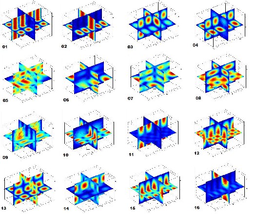
Figure 4, Electric Field Plot at Each Eigenvalue with 1Litre of Water

http://www.ijser.org

International Journal of Scientific & Engineering Research, Volume 4, Issue 9, September-2013 2476

ISSN 2229-5518

TABLE 3.2

RESONANT FREQUENCY & QUALITY FACTOR WITH

1LITRE OF WATER

Inc, Third Edition, pp. 278-282.

[3] Das, Annupurna. and Das, Sisir K. 2009, Microwave Engineering, Tata McGraw-Hill, Second Edition, pp. 186-188.

[4] Vollmer, Michael. 2004, “Physics of the Microwave Oven”, Physics

Education, vol.39, no.1, pp. 74-81.

[5] COMSOL Multiphysics 3.5 User guide [online]

http://math.nju.edu.cn/help/mathhpc/doc/comsol/guide.pdf [Accessed:

01, July 2013]

[6] Rectangular & Circular Waveguide: Equations & Fields [online] http://www.rfcafe.com/references/electrical/waveguide.htm [Accessed: 13, Sept 2011]

A huge drop into the Quality factor is observed. It was obvious that Quality factor will go down after the addi- tion of load (1Litre of water). The interesting fact would be to have an idea of how it affects the hotspots inside the cavity on each resonant frequency.

3 DISCUSSION

The plot for the first two eigenvalues almost remains the same but for the next eigenvalues the hotspots are increased and we can see a big change. This shows the affects of adding water in huge amount (1Litre). It might be because when we add huge amount of load in the microwave they turn to be more efficient, and works more into a single mode frequency. The eigenvalue 13 i.e. 2.4842 GHz frequency, a single mode frequency can be seen and therefore the hotspots are well ar- ranged all over the rectangular cavity. The most important fact that can be clearly seen and achieved is that there’s a lot hap- pening in the cavity. In the analysis, we are lucky enough to get the single mode frequency otherwise if we deviate a little bit, the whole pattern changes. For example at 2.5010 GHz, the hotspots were quiet well arranged but with the addition of water they are drastically changed. The same is the case on eigenvalues 6, 11 and 14. This shows that we have to be very precise for choosing the right bandwidth otherwise they can behave differently to our expectations.

4 CONCLUSION

A microwave oven in modeled and eigenvalues are obtained for empty and with 1 litre of load. By analyzing the results, we have established the fact that for the specific eigenvalues or resonant frequencies, it is working efficiently having some particular exceptions at certain values. It was observed that when the number of hotspots are greater in the plot we get lower value of quality factor.

REFERENCES

[1] Parker, Kerry. and Vollmer, Michael. 2004, “Bad food and good physics: the development of domestic microwave cookery”, Physics Education, vol.39, no.1, pp. 82-90.

[2] Pozar, David M. 2005, Microwave Engineering, John Wiley & Sons

IJSER © 2013 http://www.ijser.org