International Journal of Scientific & Engineering Research, Volume 6, Issue 5, May-2015 49

ISSN 2229-5518

Effect of Particles on Flow Structures in

Secondary Sedimentation

Tanks Using Neural Network Model

Mostafa Y.El-Bakry* ,D.M.Habashy** and Mahmoud Y.El-Bakry**,***

Abstract— Sedimentation tanks are designed for removal of floating solids in water flowing through the water treatment plants. These tanks are one of the most important parts of water treatment plants and their performance directly affects the functionality of these systems. Flow pattern has an important role in the design and performance improvement of sedimentation tanks. In this work, the neural network model is used to study the particle-laden flow in a rectangular sedimentation tank which used the Kaolin as solid particles. The neural network simulation has been designed to simulate and predict the Shear stress coefficient at the bottom of tank for various inlet concentrations and maximum streamwise velocity along the channel. The system was trained on the available data of the two cases. Therefore, we designed the system for finding the best network that has the ability to have the best test and prediction. The proposed system shows an excellent agreement with that of an experimental data in these cases.

Index Terms— Shear stress ,Neural networks, Maximum streamwise velocity, Rectangular sedimentation tanks, Particle-laden flows.

——————————  ——————————

1 INTRODUCTION

Solids removal is probably the main process in water purification method in filtration plants. The most significant phase of this process is the separation of sludge and suspended particles from water by means of gravity. In these basins, the turbid water flows into the basin at one end and the cleaner water is taken out at the other end by decanting. Obviously, the water must flow in the tank long enough for appropriate particles deposition. The performance of these sedimentation tanks directly affects the filtration basin’s efficiency. Sedimentation tanks are divided into two main categories. The primary settling tanks have a low influent concentration and the flow field in them is not influenced much by concentration field due to the negligible buoyancy effects. The secondary or final settling tanks have a higher influent concentration and they are usually placed after the primary and activation tanks Tamayol et al.[1]. So they usually contain activated sludge and hence, the size of particles would grow and flow field is influenced by concentration distribution. Generally, the sedimentation tanks are characterized by several hydrodynamic phenomena, such as density waterfalls, bottom current and surface return currents, and are also sensitive to temperature fluctuations and wind effects. Various studies have been conducted to find the effects of particles on the flow and hydraulics of settling tanks. Imam and McCorquodale [2]solved flow

_________________

*Physics Department, Faculty of Science, Benha

University, Egypt mail: oelbakre@yahoo.com

**Physics Department, Faculty of Education Ainshams

University

***Physics Department, Faculty of Science University of

Tabuk

equations with a constant turbulent eddy
diffusivity assumption.
Celik and Rodi [3] and Stamou and Rodi [4] used k-ε turbulence model to predict the flow field in settling tanks. Kerbs [5]developed one and two dimensional models
for clarifier modeling. He observed that worse
sludge quality causes stronger density current and thus increases the tendency for short circuiting between the inlet and the outlet. Zhou et al.[6] applied a 3-dimensional fully mass conservative clarifier model, based on modern computational fluid dynamics theory. They observed that the upward buoyant flow occurs in the tank with deep sludge blanket and a short circuiting flow appears near the water surface and flow regime is strongly affected by the sludge blanket in the tank. Mazzolani et al.[7] developed numerical models for the prediction of turbulent flow and suspended solid distribution in the sedimentation tank. They found that increasing the concentration in region between discrete settling and hindered settling, results in an increase in settling velocities of the faster particles. In addition, the application of the three distinct settling models in the numerical analysis of the transport in a rectangular sedimentation tank, yields highly different predictions of solid distribution and removal rate. On the other hand, the main features of the

International Journal of Scientific & Engineering Research, Volume 6, Issue 5, May-2015 50

ISSN 2229-5518

hydrodynamic field are qualitatively similar. Tamayol and Firoozabadi [8] studied the effects of different turbulent models on the flow field. Tamayol et al.[9] also studied the hydrodynamics of secondary settling tanks while using baffles for increasing their performance. They found that it is required to calculate the concentration profiles in the tank, as well as the velocity profiles. Also their results showed that both Reynolds and Froude numbers are important in determination of the degree of importance of buoyancy forces in sedimentation tanks. In tanks with low buoyancy forces, the problem is due to short circuiting between the inlet and outlet, while in the tanks which are highly stratified, the problematic phenomenon is bottom density currents. The design of tanks with high deposition rate and hydraulic efficiency requires complete investigation of the effect of particles on the flow hydrodynamics. In addition, the investigation of the physics of sedimentation and its effects on the hydrodynamics of sedimentation tanks are rare. Asgharzadeh et al.[10] studied the effect of particles on hydrodynamics of flow field in secondary
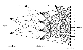
also known as processing elements (PE) as they process information. Each PE has weighted inputs, transfer function and one output. PE is essentially an equation which balances inputs and outputs. There are many types of neural networks designed by now and new ones are invented every week but all can be described by the transfer functions of their neurons, by the training or learning algorithm (rule), and by the connection formula. A single-layer neuron is not able to learn and generalize the complex problems. The multilayer perceptron (MLP) overcomes the limitation of the single-layer perceptron by the addition of one or more hidden layer(s)Fig.(1). The MLP has been proven to be a universal approximator Cybenko [27]. In Fig. (1), a feedforward multilayer perceptron network was presented. The arriving signals, called inputs, multiplied by the connection weights (adjusted) are first summed (combined) and then passed through a transfer function to produce the output for that neuron. The neuron transfer function, f, is typically step or sigmoid function that produces a scalar output(O) as follows
sedimentation tanks experimentaly and
numerically.
In this work, we introduce the artificial

O = f (

∑ Wi Ii i

+ b ) ( 1 )

neural network (ANN) for modelling the Shear stress coefficient at the bottom of tank for various inlet concentrations and Maximum streamwise velocity along the channel using the data obtained from Asgharzadeh et al.[10].
Neural networks are widely used for solving
many problems in most science problems of
linear and non-linear cases [11-20]. Neural network algorithms are always iterative, designed to step by step minimise (targeted minimal error) the difference between the actual output vector of the network and the desired output vector [21-23]. The data obtained by [10] is chosen to be carried out using the neural networks .
The present work offers neural network to simulate and predict the unknown data of the
shear stress coefficient and maximum streamwise velocity along the channel as a function of distance of at the bottom of tank at various inlet concentrations. The rest of paper is organized as follows; Sec. 2 describes the artificial neural network . Section 3 presents the proposed system. Section 4 shows the obtained results. Finally, Sec. 5 concludes the work.

2 Artificial Neural Network

Bourquin et al. [24,25] and Agatonovic- Kustrin and Beresford[26] described the basic theories of ANN modeling. An ANN is a biologically inspired computational model formed from several of single units, artificial neurons, connected with coefficients (weights) which constitute the neural structure. They are
where Ii , Wi and b are i th input, i th weight and
bias, respectively.
The activation (transfer) function acts on the
weighted sum of the neuron’s inputs and the

most commonly used transfer function is the sigmoid (logistic) function. The way that the neurons are connected to each other has a significant impact on the operation of the ANN (connection formula). There are two main connection formulas (types): feedback (recurrent) and feedforward connection. Feedback is one type of connection where the output of one layer routes back to the input of a previous layer, or to same layer. Feedforward does not have a connection back from the output to the input neurons. There are many different learning rules (algorithms) but the most often used is the Delta-rule or backpropagation (BP) rule.
Fig.(1). Schematic representation of a multilayer perceptron feedforward network
consisting of two inputs, one hidden layer with four neurons and 14 outputs.
A neural network is trained to map a set of input data by iterative adjustment of the weights.

International Journal of Scientific & Engineering Research, Volume 6, Issue 5, May-2015 51

ISSN 2229-5518

Information from inputs is fed forward through the network to optimize the weights between neurons. Optimization of the weights is made by backward propagation of the error during training or learning phase. The ANN reads the input and output values in the training data set and changes the value of the weighted links to reduce the difference between the predicted and target (observed) values. The error in prediction is minimized across many training cycles (iteration or epoch) until network reaches specified level of accuracy. A complete round of forward–backward passes and weight adjustments using all input–output pairs in the data set is called an epoch or iteration.

3 Modeling Shear Stress Coefficient and

Maximum Streamwise Velocity Using ANN

Shear stress coefficient Cd and maximum streamwise velocity Umax can be simulated and
predicted at different inputs using ANN. we
choose to internally model the problem with two
individual neural networks trained separately
using experimental data. The first ANN was
configured to have distance at bottom tank X/Lo and Cin (0,400 and 800) as inputs while the output is Shear stress coefficient Cd . The second
learning of the network i.e. when ΔW tends to zero this means that the network has been learnt (ready to predict the unseen values).Then the adjustment for the weights is done by Eq. (2) to reduce the error value.

4 Results

The proposed ANN models were applied to
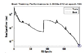
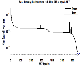
simulate the shear stress coefficient Cd (referred to as model1) and maximum streamwise velocity Umax (model 2). By employing the above mentioned proposed models with different values of the ANN parameters we have obtained different numbers of hidden neurons for the ANN models. The results obtained by the two models are discussed in the following: The first ANN having three hidden layers of 67 , 86 and
94 neurons (model1) and second network having
90 , 77 and 80 neurons(model2) respectively with
one neuron in the output layer. Network performance was evaluated by plotting the ANN model output against the experimental data and analyzing the percentage error between the simulation results and the experimental data Fig. (3). In the training process, 196 and 657 epochs was found to be sufficient, Fig. (3), with respect to the minimum mean sum square error (MSE)
ANN was configured to have distance at bottom

-12

of 2.3939×10

-13

and 9.8191×10
respectively. For
tank X/Lo and C in (0,400 and 800) as inputs
while the output is maximum streamwise velocity Umax . Fig.(2) represent a block diagram of the two ANN based modeling.
all networks, the function which describes the nonlinear relationship is given in appendix.
(a)

Distance at bottom tank X/Lo

Inlet concentration

Cin

Distance at bottom tank X/Lo

Inlet concentration

Cin

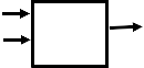
ANN

Shear stress coefficient Cd

Maximum streamwise velocity Umax

Fig.(2): Block diagram of the two ANN based modeling.
The performance of the previous two models is examined by using the mean square error (MSE) .The proposed ANN was trained using the Levenberg–Marquardt optimization technique. This optimization technique is more powerful than the conventional gradient descent techniques. The Levenberg– Marquardt updates the net- work weights using the following rule:
ΔW=(JTJ+µI)-1JTe (2)
where J is the Jacobian matrix of derivatives of
each error with respect to each weight; JT is the
transposed matrix of J; I is the identity matrix that
has the same dimensions as those of JTJ; µ is a
scalar changed adaptively by the algorithm and e is an error vector. ΔW is a measure for the rate of

(b)
Fig. 3: Performance using ANN model, where epochs are the number of training

International Journal of Scientific & Engineering Research, Volume 6, Issue 5, May-2015 52

ISSN 2229-5518

(a) Shear stress coefficient Cd

(b) Maximum streamwise velocity

Umax
The above mentioned details of the proposed
ANN model (model1) are carried out and simulated two the experimental data of the distance at bottom tank X/Lo and Shear stress coefficient Cd using the obtained function which is given in appendix. The proposed Cd is trained using ANN model on three cases of inlet concentration Cin . The values of these cases are 0,
400 and 800 Fig.(4) . After the training , the obtained system is predicted the behavior of inlet concentration Cin =1000 Fig.(4). It is found that as shown in Fig. (4), the obtained results (simulated

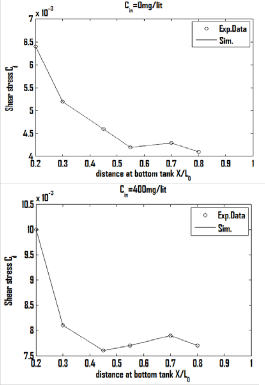
and predicted) are provided to demonstrate good agreement with the experimental data[10] .

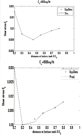
Fig. 4. ANN simulation and prediction of shear stress coefficient.
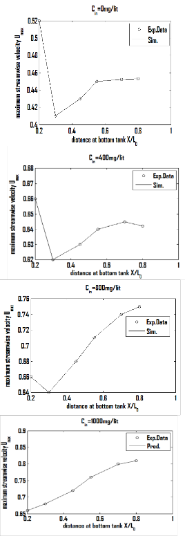
Also, ANNs are chosen to be applied on the maximum streamwise velocity Umax (model2) at different values of inlet concentration Cin . The training values inlet concentration Cin are 0, 400 and 800 as shown in Fig.(5). The predicted value of inlet concentration Cin = 1000 is in Fig(5). The simulation and predicted results from the obtained function which is given in appendix are best fitting with the experimental data. It is noted from Fig(4) and Fig(5) that, the proposed ANN model shows excellent results matched well the experimental data.

International Journal of Scientific & Engineering Research, Volume 6, Issue 5, May-2015 53

ISSN 2229-5518

predicted methods was investigated in several cases to ensure the effectiveness to establish the results with less permissible error. It can be concluded by analyzing the results that the artificial neural network can predict the shear stress coefficient Cd at the bottom of tank for various inlet concentrations and maximum streamwise velocity along the channel Umax accurately with minimum relative error. The trained ANN network shows excellent results matched with the experimental data in the two cases of the shear stress coefficient Cd and maximum streamwise velocity Umax . The designed ANN introduce a powerful model and shows a good match to the experimental data. Then, the capability of the ANN techniques to simulate and predict the experimental data with almost exact accuracy recommends the ANN to dominate the modelling techniques in fluid mechanics.

Appendix

The equation which describe shear stress
coefficient and maximum streamwise velocity is
given by:

CRdR and URmaxR =Pureline [net. LW{4,3} logsig(net. LW{3,2} logsig(net.LW{2,1} logsig(net. IW{1,1} A

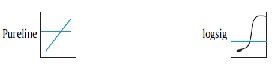
+net. b{1})+net. b{2})+net. b{3})+net. b{4}], Where

A =X/LRoR is the input

net. IW{1,1}: linked weights between the input layer and first hidden layer.
net. LW{2,1}: linked weights between the first hidden layer and the second hidden layer.
net. LW{3,2}: linked weights between the second
hidden layer and third layer.
net. LW{4,3}: linked weights between the third
hidden layer and output layer.
net . b{1}: is the bias of the first hidden layer.
net . b{2}: is the bias of the second hidden layer.
net . b{3}: is the bias of the output layer. net. b{4}: the bias of the output layer.
Fig. 5. ANN simulation and prediction of maximum streamwise velocity Umax

5 Conclusion

In this work, a method was proposed to model the Shear stress coefficient Cd at the bottom of tank for various inlet concentrations and maximum streamwise velocity along the channel Umax using ANN. For training and testing the network, several numerical cases with combinations of input variables and output data are generated. The validity of the applied

References:

1. Tamayol, A., Firoozabadi B. and Ahmadi G. (2008).Effects of Inlet Position and Baffle Configuration on Hydraulic Performance of Primary Settling Tanks. Journal of Hydraulic Engineering, ASCE 134(7), 1004-1009.
2. Imam, E. and McCorquodale J.A. (1983).
Simulation of Flow in Rectangular
Clarifiers. Journal of Environmental

Engineering 109(30), 713-730.

3. Celik, I. and Rodi W. (1985). Prediction of Hydrodynamic Characteristics of Rectangular Settling Tanks. Int. Symp.

International Journal of Scientific & Engineering Research, Volume 6, Issue 5, May-2015 54

ISSN 2229-5518

On Refined Flow Modeling and Turbulence

Measurements 20(1), 641–665.

4. Stamou, C.R and Rodi W. (1990).
Evaluating the Effect of Geometrical
Modification on the Hydraulic
Efficiency of Water Tanks Using Flow
Through Curves and Mathematical Models. Journal of Hydro Informatics, ASCE 20(1), 77-83.
5. Kerbs, P. (1995). Success and
Shortcomings of Clarifier Modeling.

Wat. Sci. Tech. 2(31), 181-191.

6. Zhou, S., C. Vitasovic, J.A.
McCorquodale, S. Lipke, M. DeNicola,
and P. Saurer, (1997). Improving
Performance of Large Rectangular
Secondary Clarifiers. Proceedings of the

70th Annual WEF Conference and

Exposition, Chicago, USA.

7. Mazzolani, G., Pirozzi F. and Antoni G.D. (1998). A Generalized Settling Approach in the Numerical Modeling of Sedimentation Tanks. Wat. Sci. Tech.
3(38), 95-102.
8. Tamayol A., and Firoozabadi B. (2006).
Effects of Turbulent Models and Baffle
Position on Hydrodynamics of Settling
Tanks. Scientia Iranica 13(3), 255–260.
9. Tamayol, A., Firoozabadi B. and Ashjari
M. A. (2010). Hydrodynamics of Secondary Settling Tanks and Increasing Their Performance Using Baffles. Journal of Environmental Engineering, ASCE
136(1), 32-39.
10. Asgharzadeh H., Firoozabadi B. and
Afshin H. (2012). Experimental and
Numerical Simulation of the Effect of
Particles on Flow Structures in Secondary Sedimentation Tanks. Journal of Applied Fluid Mechanics, Vol. 5, No.
2,15-23.
11. El-Bakry Mostafa.Y.,Habash D.M. and
El-Bakry Mahmoud Y. (2014).Neural Network Model for Drag coefficient and Nusselt number of square prism placed inside a wind tunnel. International Journal of Sc.&Eng.Reasearch, Vol.(5) Issue 6, 1411-1417.
12. El-Bakry Mostafa.Y.,(2011), Radial Basis Function Neural Network Model for Mean velocity and Vorticity of Capillary Flow, Inter. J.for numerical methods in fluids 67:1283-1290.
13. El-Bakry Mostafa.Y., El-Bakry Mahmoud Y. and Elhelly M. (2009) "Neural Network Represntation For the Forces and Torque of The Eccentric Sphere Model, Trans.on Comput.Sci.III,LNCS 5300,pp171-183.
14. El-Bakry Mostafa.Y., A., El-Harby A.
and Behery G. M. (2008). Automatic
Neural Network System for Vorticity of
Square Cylinders With Different Corner Radii, Journal of Applied Mathematics And Informative(JAMI),Vol.26, No.5-6, pp911-923
15. Behery G.M., El-Harby A.A. and.El-
Bakry Mostafa.Y. (2009). Reorganizing
Neural Network System for Two-Spirals
and Linear-Low-Density Polyethylene
Copolymer problems, Applied Computational Intelligence and soft computing. Volume 2009, Article ID
721370, 11 pages.
16. El Bakry M.Y. and El-Metwally K. A.
(2003). "Neural Network for Proton-
Proton Collision at High Energy", Chaos, Solitons and Fractals, vol. 16, No.
2, pp. 279-285.
17. El Bakry M.Y. (2003). "Feed Forward
Neural Networks Modeling for K-P
Interactions", Chaos, Solitons and
Fractals, vol. 16, No.2, pp. 279-285.
18. Scalabrin G., Corbetti C. and Cristofoli
G. (2001). "A Viscosity Equation of state
for R123 in the form of a Multilayer feed
forward Neural Network" Inter.J. of
Thermophyscis, vol. 22, No.5.
19. El-dahshan E., Radi A. and El-Bakry M.
Y. (2008). Artificial Neural Network and
Genetic Algorithm Haybrid Technique
for Nucleus-Nucleus Collisions; Int. J.
Mod Phys C 19, 1787 .
20. Latafat A. Gardashova (2014).
Application of DEO Method to Solving
Fuzzy Multiobjective Optimal Control
Problem, Applied Computational
Intelligence and Soft Computing, Article
ID 971894, Volume 2014, 7 pages.
21. Yi-Chung Hu, and Jung-Fa Tsai (2006).
"Backpropagation multi-layer
perceptron for incomplete pairwise
comparison matrices in analytic hierarchy process", Applied Mathematics and Computation, vol. 180, No. 1, pp. 53-62 .
22. Curry B., and Morgan P.H.(2004) "Model
selection in Neural Networks: Some difficulties", European Journal of Operational Research, vol. 170, No.
2, pp. 567-577.
23. Jochen J. Steil, (2006)."Online stability of
Backpropagation–decorrelation
recurrent learning" Neurocomputing, vol. 69, No. 7-9, pp.
642-650
24. A. Ghaffari et al. (2006).International
Journal of Pharmaceutics ,327,pp 126–
138.
25. Bourquin, J., Schmidli, H., Hoogevest,
P.V., Leuenberger, H. ( 1997). Basic
concepts of artificial neural networks
(ANN) modeling in the application to

International Journal of Scientific & Engineering Research, Volume 6, Issue 5, May-2015 55

ISSN 2229-5518

pharmaceutical development. Pharm. Dev. Tech. 2,pp 95–109.
26. Agatonovic-Kustrin, S., Beresford, R. (2000). Basic concepts of artificial neural network (ANN) modeling and its
application in pharmaceutical research. J. Pharm. Biomed. Anal. 22, pp 717–727.
27. Cybenko, G. (1989). Approximation by superposition of a sigmoidal function. Math. Control Signals Syst. 2,pp 303–
314.