robustness toward changes on demands. Through illu- strative simulations with variation of demand, it is dem- onstrated that move suppression effect decreases maxi- mum changes of customer demands.
International Journal of Scientific & Engineering Research Volume 2, Issue 5, May-2011 1
ISSN 2229-5518
Decreasing Inventory Levels Fluctuations by Moving Horizon Control Method and Move Suppression in the Demand Network
Mohammad Miranbeigi, Aliakbar Jalali
—————————— • ——————————
ey elements to an efficient supply chain are accurate pinpointing of process flows and timing of supply needs at each entity, both of which enable entities to request items as they are needed, thereby reducing safety stock levels to free space and capital. The operational planning and direct control of the network can in prin- ciple be addressed by a variety of methods, including deterministic analytical models and stochastic analytical models, and simulation models, coupled with the desired optimization objectives and network performance meas-
ures [1].
The significance of the basic idea implicit in the moving
horizon control (MHC) or MHC has been recognized a
long time ago in the operations management literature as a tractable scheme for solving stochastic multi period op- timization problems, such as production planning and supply chain management, under the term moving hori-
zon [2]. In a recent paper [3], a MHC strategy was em- ployed for the optimization of production/distribution systems, including a simplified scheduling model for the manufacturing function. The suggested control strategy considers only deterministic type of demand, which re- duces the need for an inventory control mechanism [4,5].
For the purposes of our study and the time scales of in- terest, a discrete time difference model is developed [6]. The model is applicable to multi echelon supply chain networks of arbitrary structure. To treat process uncer- tainty within the deterministic supply chain network
————————————————
Mohammad Miranbeigi is currently pursuing Phd degree program in control engineering in University of Tehran, Iran, E-mail: m.miran@ut.ac.ir
A. A. Jalali, is associate professor in the Department of Electrical Engi-
neering, Iran University of Science and Technology, Narmak ,Tehran, Iran, E-mail : drjalali@iust.ac.ir.
model, a MHC approach is suggested [7,8].
Typically, MHC is implemented in a centralized fa- shion [9]. The algorithm uses a moving horizon, to allow the incorporation of past and present control actions to future predictions [10,11,12,13].
In this paper, a moving horizon controller with move suppression term used for inventory management of the demand network.
In this work, a discrete time difference model is devel- oped[4]. The model is applicable to multi echelon supply chain networks of arbitrary structure, that DP denote the set of desired products in the supply Chain and these can be manufactured at plants, P, by utilizing various re- sources, RS. The manufacturing function considers inde- pendent production lines for the distributed products. The products are subsequently transported to and stored at warehouses, W. Products from warehouses are trans- ported upon customer demand, either to distribution cen- ters, D, or directly to retailers, R. Retailers receive time varying orders from different customers for different products. Satisfaction of customer demand is the primary target in the supply chain management mechanism. Un- satisfied demand is recorded as backorders for the next time period. A discrete time difference model is used for description of the supply chain network dynamics. It is assumed that decisions are taken within equally spaced time periods (e.g. hours, days, or weeks). The duration of the base time period depends on the dynamic characteris- tics of the network. As a result, dynamics of higher fre- quency than that of the selected time scale are considered negligible and completely attenuated by the network [4,14]. Plants P, warehouses W, distribution centers D, and retailers R constitute the nodes of the system. For each node, k, there is a set of upstream nodes and a set of
IJSER © 2011 http://www.ijser.org
International Journal of Scientific & Engineering Research Volume 2, Issue 5, May-2011 2
ISSN 2229-5518
downstream nodes, indexed by (k ', k '') . Upstream nodes can supply node k and downstream nodes can be sup-
MHC originated in the late seventies and has devel- oped considerably since then. The term MHC does not
plied by k. All valid (k ', k )
and/or
(k , k ' ) pairs constitute
designate a specific control strategy but rather an ample
permissible routes within the network. All variables in the supply chain network (e.g. inventory, transportation loads) valid for bulk commodities and products. For unit products, continuous variables can still be utilized, with the addition of a post processing rounding step to identi- fy neighbouring integer solutions. This approach, though clearly not formally optimal, may be necessary to retain computational tractability in systems of industrial relev- ance.
A product balance around any network node involves the inventory level in the node at time instances t and t -
1, as well as the total inflow of products from upstream nodes and total outflow to downstream nodes. The fol- lowing balance equation is valid for nodes that are either warehouses or distribution centers:
yi,k (t) = yi,k (t -1) + xi,k',k (t - Lk ',k ) - xi,k,k'' (t),
range of control methods which make explicit use of a model of the process to obtain the control signal by mi- nimizing an objective function. The ideas, appearing in greater or lesser degree in the predictive control family, are basically the explicit use of a model to predict the process output at future time instants (horizon), the calcu- lation of a control sequence minimizing an objective func- tion and the use of a moving strategy, so that at each in- stant the horizon is displaced towards the future, which involves the application of the first control signal of the sequence calculated at each step. The success of MHC is due to the fact that it is perhaps the most general way of posing the control problem in the time domain. The use a finite horizon strategy allows the explicit handling of process and operational constraints by the MHC. The con- trol system aims at operating the supply chain at the op- timal point despite the influence of demand changes
k {W, D},
k'
t T,
k '
i DP
(1)
[12,13]. The control system is required to possess built in
capabilities to recognize the optimal operating policy
through meaningful and descriptive cost performance
indicators and mechanisms to successfully alleviate the
where
yi, k is the inventory of product i stored in node
detrimental effects of demand uncertainty and variability. The main objectives of the control strategy for the supply
k; xi,k ',k denotes the amount of the i-th product trans-
chain network can be summarized as follows: (i) maxim-
ported through route (k ', k ) ;
Lk ',k denotes the transporta-
ize customer satisfaction, and (ii) minimize supply chain
tion lag (delay time) for route (k ', k ) , i.e. the required time
periods for the transfer of material from the supplying node to the current node. The transportation lag is as- sumed to be an integer multiple of the base time period.
For retailer nodes, the inventory balance is slightly
modified to account for the actual delivery of the i-th product attained, denoted by di,k (t) .
yi,k (t ) = yi, k (t - 1) + xi, k ' ,k (t - Lk ' ,k ) - di,k (t ),
operating costs.
The first target can be attained by the minimization of back orders (i.e. unsatisfied demand) over a time period because unsatisfied demand would have a strong impact on company reputation and subsequently on future de-
mand and total revenues. The second goal can be achieved by the minimization of the operating costs that include transportation and inventory costs that can be further divided into storage costs and inventory assets in the supply chain network. Based on the fact that past and
k {R},
k '
t T ,
i DP.
(2)
present control actions affect the future response of the system, a moving time horizon is selected. Over the speci- fied time horizon the future behavior of the supply chain
The amount of unsatisfied demand is recorded as back- orders for each product and time period. Hence, the bal- ance equation for back orders takes the following form:
BOi,k (t) = BOi,k (t -1) + Ri,k (t) - di,k (t) - LOi,k (t),
is predicted using the described difference model (Eqs. (1)–(3)). In this model, the state variables are the product inventory levels at the storage nodes, y, and the back or- ders, BO, at the order receiving nodes. The manipulated (control or decision) variables are the product quantities
k {R},
t T,
i DP.
(3)
transferred through the network’s permissible routes, x,
and the delivered amounts to customers, d. Finally, the
product back orders, BO, are also matched to the output
where Ri,k denotes the demand for the i-th product at the
variables. The inventory target levels (e.g. inventory set-
k-th retailer node and time period t.
LOi,k denotes the
points) are time invariant parameters. The control actions
amount of cancelled back orders (lost orders) because the
network failed to satisfy them within a reasonable time
limit. Lost orders are usually expressed as a percentage of
unsatisfied demand at time t. Note that the model does
not require a separate balance for customer orders at
nodes other than the final retailer nodes [4,15].
that minimize a performance index associated with the
outlined control objectives are then calculated over the
moving time horizon. At each time period the first control action in the calculated sequence is implemented. The effect of unmeasured demand disturbances and model mismatch is computed through comparison of the actual
IJSER © 2011 http://www.ijser.org
International Journal of Scientific & Engineering Research Volume 2, Issue 5, May-2011 3
ISSN 2229-5518
current demand value and the prediction from a stochas- tic disturbance model for the demand variability. The difference that describes the overall demand uncertainty and system variability is fed back into the MHC scheme at each time period facilitating the corrective action that is required.
The centralized mathematical formulation of the per- formance index considering simultaneously back orders, transportation and inventory costs takes the following form[4]:
J total =
t + P
wy ,i, k ( yi, k (t ) - ys ,i, k (t ))2
t k {W , D , R}i DP
judged and selected mainly on grounds of desirable achieved performance.
The weighting factors in cost function also reflect the
relative importance between the controlled (back orders
and inventories) and manipulated (transported products)
variables. Note that the performance index of cost func-
tion reflects the implicit assumption of a constant profit
margin for each product or product family. As a result, production costs and revenues are not included in the index.
In this centralized implementation, MHC will opti- mized for whole policy and then will sent downstream optimal inputs to upstream joint nodes to those nodes which it is coupled, as measurable disturbances.
t + M
+
{w ' ( x
' (t ))2 }
(4)
Each node completely by a centralized MHC optimizes
for whole policy. At each time period, the first control
t
t + P
k {W , D , R }i DP
x ,i, k , k
i, k ,k
action in the calculated sequence is implemented until
MHC process complete.
+
t
t + M
k {R}i DP
{wBO ,i ,k ( BOi ,k (t))2 }
+ {w
' ( x
' (t ) - x
' (t - 1))2 }.
t k {W , D , R }i DP
�x,i , k , k
i, k , k
i ,k , k
A four echelon supply chain system is used in the si- mulated examples. The supply chain network consists of
The performance index, J, in compliance with the out- lined control objectives consists of four quadratic terms. Two terms account for inventory and transportation costs throughout the supply chain over the specified prediction and control horizons (P , M). A term penalizes back or- ders for all products at all order receiving nodes (e.g. re- tailers) over the moving horizon P. Also a term penalizes deviations for the decision variables (i.e. transported product quantities) from the corresponding value in the previous time period over the control horizon M. The term is equivalent to a penalty on the rate of change in the manipulated variables and can be viewed as a move sup- pression term for the control system. Such a policy tends to eliminate abrupt and aggressive control actions and subsequently, safeguard the network from saturation and undesired excessive variability induced by sudden de- mand changes. In addition, transportation activities are usually preferred to resume a somewhat constant level rather than fluctuate from one time period to another.
However, the move suppression term would definite- ly affect control performance leading to a more sluggish dynamic response. The weighting factors, w y,i ,k , reflect the
one product, two production nodes, two warehouses, four distribution centers, and four retailer nodes.
All possible connections between immediately succes- sive echelons are permitted. One product is being distri- buted through the network. Inventory setpoints, maxi- mum storage capacities at every node, and transportation cost data for each supplying route are reported in Table 1.
A prediction horizon of 20 time periods and a control horizon of 10 time periods were selected and was consi- dered LO = 3 for every times. So each delay was replaced by its 4th order Pade approximation.
Table 1. Supply chain data
L J
inventory storage costs and inventory assets per unit
product,
wx,i,k',k , account for the transportation cost per
unit product for route (k ', k ) .Weights
wBO,i,k
correspond
to the penalty imposed on unsatisfied demand and are
estimated based on the impact service level has on the company reputation and future demand. Weights w�x,i,k',k , are associated with the penalty on the rate of change for the transferred amount of the i-th
product through route (k ', k ) . Even though, factors
w y,i ,k ,
wx,i,k',k and
wBO,i,k
are cost related that can be estimated
with a relatively good accuracy, factors
w�x,i,k',k
are
IJSER © 2011 http://www.ijser.org
International Journal of Scientific & Engineering Research Volume 2, Issue 5, May-2011 4
ISSN 2229-5518
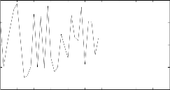
The simulated scenarios lasted for 50 time periods. Va- riant demand is presented in Fig. 1. The move suppres- sion term would definitely affect control performance leading to a more sluggish dynamic response. In this part, centralized MHC method is applied to the supply chain network with a variant customer demand that is seeing in figures 2 and 3.
robustness toward changes on demands. Through illu- strative simulations with variation of demand, it is dem- onstrated that move suppression effect decreases maxi- mum changes of customer demands.![]()
400
x(daltaU)
200 x
200
150
100
50
0
600
0 5 10 15 20 25 30 35 40 45 50
Time (days)
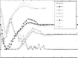
Fig. 1 Demand
W (deltaU)
0
200
100
0
200
100
0
200
100
0
0 5 10 15 20 25 30 35 40 45 50
![]()
0 5 10 15 20 25 30 35 40 45 50
![]()
0 5 10 15 20 25 30 35 40 45 50
![]()
0 5 10 15 20 25 30 35 40 45 50
Time (day s)
500
400
300
200
100
0
D(deltaU) R(deltaU)
BO(deltaU)
W
D
R BO
Fig. 3 MHC inputs of supply chain management system:deltaU
curves is with move suppression effect
[1] M. Beamon, “Supply chain design and analysis: models and
Methods”. International Journal of Production Economics, 55, pp.
281, 1998.
[2] S. Igor , “Model predictive functional control for processes with
unstable poles”. Asian journal of control,vol 10, pp. 507-513, 2008. [3] E . Perea-Lopez, , B. E . Ydstie, “ A model predictive control strategy for supply chain optimization”. Computers and Chemical Engineer-
-100
0 5 10 15 20 25 30 35 40 45 50
Time (days)
Fig. 2 MHC outputs of supply chain management system:deltaU
curves is with move suppression effect
The large majority of successful MHC applications ad- dress the case of multivariable control in the presence of constraints, motivating its extensive distribution for ap- plications where traditional control usually comes close to its limits. The success of MHC is due to the fact that it is perhaps the most general way of posing the control prob- lem in the time domain. The use a finite horizon strategy allows the explicit handling of process and operational constraints by the MHC. Typically, MHC is implemented in a centralized fashion. In this paper, a centralized mov- ing horizon controller applying to a supply chain man- agement system consist of one plant (supplier), two dis- tribution centers and three retailers. Also a move sup- pression term add to cost function, that increase system
ing, 27, pp. 1201, 2003.
[4] P. Seferlis, N. F. Giannelos, “A two layered optimization based control sterategy for multi echelon supply chain network”, Computers and Chemical Engineering, vol. 28 , pp. 799–809, 2004.
[5] G. Kapsiotis , S. Tzafestas, “ Decision making for invento-
ry/production planning using model based predictive control,” Parallel and distributed computing in engineering systems. Amster- dam: Elsevier, pp. 551–556, 1992.
[6] S. Tzafestas , G. Kapsiotis , “Model-based predictive control for
generalized production planning problems,” Computers in Industry,
vol. 34, pp. 201–210, 1997.
[7] W. Wang, R. Rivera , “A novel model predictive control algorithm
for supply chain management in semiconductor manufacturing,” Pro- ceedings of the American control conference, vol. 1, pp. 208–213,
2005.
[8] S. Chopra, P. Meindl, Supply Chain Management Strategy, Planning
and Operations, Pearson Prentice Hall Press, New Jersey, pp. 58-79,
2004.
[9] H. Sarimveis, P. Patrinos, D. Tarantilis, T. Kiranoudis, “Dy- namic modeling and control of supply chain systems: A re- view,” Computers & Operations Researc, vol. 35, pp. 3530 – 3561,
2008.
[10] E. F. Camacho, C. Bordons, Model Predictive Control. Springer,
2004.
[11] R. Findeisen, F. Allgöwer, L. T. Biegler, Assessment and future di- rections of nonlinear model predictive control, Springer, 2007.
[12] P. S. Agachi, Z. K. Nagy, M. V. Cristea, A. Imre-Lucaci, Model
Based Control, WILEY-VCH Verlag GmbH & Co, 2009.
IJSER © 2011 http://www.ijser.org
International Journal of Scientific & Engineering Research Volume 2, Issue 5, May-2011 5
ISSN 222S-5518
(13) R. Towill, "Dynamic Analysis of An Inventory and Order Based
Production Control System," Int. J. Prod. Res, vol. 20, pp. 671-
687,2008.
(14) E. Perea, "DJ11amic Modeling and Classical Control Theory for Supply Chain Management," Computers and Chemical Engineering, vol.24,pp.1143-1149,2007.
[15) J. D. Sterman , Business Dynamics Systems Thinking and Modelling
inA Complex World, Mcgraw Hill Press, pp.113-128, 2002.
IJSER 2011