International Journal of Scientific & Engineering Research Volume 2, Issue 5, May-2011 1

ISSN 2229-5518

Crank-Nicolson Scheme for Numerical Solutions of Two-dimensional Coupled Burgers’ Equations

Vineet Kumar Srivastava, Mohammad Tamsir, Utkarsh Bhardwaj, YVSS Sanyasiraju

Abstract— The two-dimensional Burgers’ equation is a mathematical model to describe various kinds of phenomena such as turbulence and viscous fluid. In this paper, Crank-Nicolson finite-difference method is used to handle such problem. The proposed scheme forms a system of nonlinear algebraic difference equations to be solved at each time step. To linearize the non-linear system of equations, Newton’s method is used. The obtained linear system is then solved by Gauss elimination with partial pivoting. The proposed scheme is unconditionally stable and second order accurate in both space and time. Numerical results are compared with those of exact solutions and other available results for different values of Reynolds number. The proposed method can be easily implemented for solving nonlinear problems evolving in several branches of engineering and science.

Keywords — Burgers’ equations; Crank-Nicolson scheme; finite- difference; Newton’s method; Reynolds number

—————————— • ——————————

1 INTRODUCTION

HE nonlinear coupled Burgers’ equation is a special form of incompressible Navier-Stokes equation with- out having pressure term and continuity equation.
Burgers’ equation is an important partial differential equ-
ation from fluid dynamics, and is widely used for various
physical applications, such as modeling of gas dynamics
and traffic flow, shock waves [1], investigating the shal-
dimensional Burgers’ equations, a detailed survey of the numerical schemes for solving the one-dimensional Burg- ers’ equation is not necessary. Interested readers can refer to [8-14] for more details.
Consider two-dimensional coupled nonlinear Burgers’
equations
low water waves[2,3], in examining the chemical reaction- au

au au

1 a 2u

a 2u

diffusion model of Brusselator[4] etc. It is also used to test several numerical algorithms. The first attempt to solve Burgers’ equation analytically was given by Bateman [5],

+ u + v ( + ) = 0, (1)

at ax ay Re ax2 ay 2

who derived the steady solution for a simple one- av

av av

1 a 2v

a 2v

dimensional Burgers’ equation, which was used by J.M. Burger in [6] to model turbulence. In the past several years, numerical solution to one-dimensional Burgers’ equation and system of multidimensional Burgers’ equa- tions have attracted a lot of attention and which has re- sulted in various finite-difference, finite-element and boundary element methods. Finite difference methods can be classified in two broad categories, i.e. explicit and implicit. Chabak and Sharma [7] have executed the solu- tion of two dimensional coupled wave eqution explicitly. An implicit approach has been utilized for solving two

+ u + v ( + ) = 0, (2)

at ax ay Re ax2 ay 2

subject to the initial conditions

u ( x , y , 0 ) = \jf 1 ( x , y ); (x , y ) E n ,

v ( x, y , 0 ) = \jf 2 ( x , y ); (x , y ) E n ,

and boundary conditions
dimensional coupled Burgers’ equations. Since in this paper the focus is numerical solutions of the two-

u ( x, y , t ) = � ( x, y , t ); (x, y ) E an,

v ( x, y , t ) = (, ( x, y , t ); (x, y ) E an ,

t > 0,

t > 0,

————————————————

Where

n = {( x, y) : a x b, c y d } and an is

• Vineet Kumar Srivastava, Faculty member, Department of Mathematics,

The ICFAI University, Dehradun, India, Email: vineetsriiitm@gmail.com

its boundary;

u( x, y, t ) and

v( x, y, t ) are the velocity

• Mohammad Tamsir, Faculty member, Department of Mathematics, The

ICFAI University, Dehradun, India, Email: tamsiriitm@gmail.com.

• Utkarsh Bhardwaj, third year B.Tech. Computer Science student, Depart-

ment of Computer Science, The ICFAI University, Dehradun, India, Email:

hap_tork@hotmail.com.

• YVSS Sanyasiraju, Professor, Department of Mathematics, IIT Madras

Chennai, India. E-mail: sryedida@iitm.ac.in.

components to be determined,\jf 1 ,\jf 2 , � and (, are
known functions and Re is the Reynolds number.
The analytic solution of eqns. (1) and (2) was proposed by
Fletcher using the Hopf-Cole transformation [15]. The
numerical solutions of this system of equations have been

IJSER © 2011 http://www.ijser.org

International Journal of Scientific & Engineering Research Volume 2, Issue 5, May-2011 2

ISSN 2229-5518

solved by many researchers. Jain and Holla [16] devel-

1 n +1

2 n+1

n +1

n 2 n n

oped two algorithms based on cubic spline method.

v

+ {( i , j +1

vi , j + vi, j 1 ) + ( vi , j +1

vi , j + vi, j 1 )}] = 0

Fletcher [17] has discussed the comparison of a number of different numerical approaches.Wubs and Goede [18] have applied an explicit–implicit method. Goyon [19] used several multilevel schemes with ADI. Recently A. R. Bahad1r [20] has applied a fully implicit method.

2 ( y)2 ( y)2

Consider the above nonlinear system of equations in the form
In this paper, Crank-Nicolson finite-difference scheme is
used for solving two-dimensional coupled nonlinear

e ( w ) =

Where,

0 , ( 3 )

( , ,........, )t ,

Burgers’ equations. Two numerical examples have been

e= g1 g2

g2 n

carried out and their results are presented to illustrate the efficiency of the proposed method.

w = (u n +1 , vn +1 , u n +1 , vn +1 ,........, u n +1 , v n +1 ),

1 1 2 2 n n

and

n = nx

1 = ny

1. Newton’s method when it is ap-

2 THE SOLUTION PROCEDURE

The computational domain n is discretized with uniform grid. Denote the discrete approximation of u( x, y, t ) and

plied to (3) results in the following steps:
1. set w( 0) , an initial approximation.
2. while for k = 0,1, ....... until convergence do:

( k ) ( k ) ( k )

v( x, y, t ) at the grid point (i x, j y, n t ) by

u n and

• solve J (w

) w

= e(w ),

vn respectively (i = 0,1, 2......, n ; j = 0,1, 2....., n ;

• set w( k +1) = w( k ) + w( k ) ,

( k )

( k )

n = 0,1, 2......), where

x = 1/ nx

is the grid size in x-
Where

J (w

) is the Jacobian matrix and w

is the cor-
direction,

y = 1/ ny

is the grid size in y-direction, and

rection vector. It is a n x n square matrix whose elements are

blocks of size 2 x 2 . Newton’s iteration at each time-step is

t represents the increment in time.

Crank-Nicolson finite-difference approximation to (1) is given by

stopped when || e(w( k ) ) || 10 5 .

By using Taylor’s series expansion one can easily see that the present scheme has accuracy of order

n+1

n n+1

n+1

n n O(( t )2 + ( x)2 + ( y)2 ) .

ui , j

ui , j + 1 [ u n+1 ( ui +1, j

ui 1, j ) + u n ( ui +1, j

ui 1, j ) ]

t 2

i , j

2 x

i, j

2 x

+ 1 [ vn+1 ( ui , j +1

ui , j 1 ) + vn

u

( i , j +1

ui , j 1 ) ]

3 NUMERICAL EXAMPLES AND DISCUSSION

2 i , j

n+1

2 y

n +1

i , j

n n

2 y

3.1 Problem 1

The exact solutions of Burgers’ equations (1) and (2) can

1 1 n +1

2 n+1

n +1

n 2 n n

u

[ {( i+1, j

ui , j

+ ui 1, j ) + ( ui +1, j

ui , j + ui 1, j )}

be generated by using the Hopf–Cole transformation [13]

Re 2 ( x)2

( x)2

which are:

u( x, y, t ) = 3 1 ,

1 n+1

2 n +1

n+1

n 2 n n

4 4[1 + exp( ( 4x + 4 y t) Re/ 32 )]

u

+ {( i , j +1

ui, j

+ ui , j 1 ) + ( ui, j +1

ui, j + ui, j 1 )}] = 0

2 ( y)2

( y)2

v( x, y, t) = 3 + 1 ,

4 4[1 + exp( ( 4 x + 4 y t ) Re/ 32 )]

Similarly, Crank-Nicolson approximation to (2) is given
Here the computational domain is taken as a square do-

by main n = {( x, y) : 0

x 1, 0

y 1} . The initial and

n +1

n n +1

n +1

n n boundary conditions for u( x, y, t ) and v( x, y, t ) are tak-

vi , j

vi , j + 1 [ u n +1 ( vi +1, j

vi 1, j ) + u n

v

( i +1, j

vi 1, j ) ]

t 2

n+1

i , j

n +1

2 x

i , j

n n

2 x

en from the analytical solutions. The numerical computa-

tions are performed using uniform grid, with a mesh width x = y = 0.05 . From Tables 1-10, it is clear that

+ 1 [ vn+1 ( vi , j +1

vi , j 1 ) + vn

v

( i , j +1

vi , j 1 ) ]

the results from the present study are in good agreement

2 i , j

1 1 n+1

2 y

2 n +1

i , j

n+1

2 y

n 2 n n

with the exact solution for different values of Reynolds number. From Tables 1-10, it is also clear that that the

v

[ {( i +1, j

vi , j

+ vi 1, j ) + ( vi +1, j

vi , j + vi 1, j )}

present scheme is unconditionally stable as it is accurate

Re 2 ( x)2

( x)2

for any time step-size. Perspective views of u and v for

Re=500 at t = 0.5 with t = 0.001 are given in Figs.

1 and 2.

IJSER © 2011 http://www.ijser.org

International Journal of Scientific & Engineering Research Volume 2, Issue 5, May-2011 3

ISSN 2229-5518

Table 2
The numerical results for v in comparion with the exact solu-

3.2 Problem 2.

tion at t = 0.5 and t = 2 with

t = 0.0001 , and Re = 10 .

Here the computational domain is taken as
(x, y) t=0.5 t=2

n = {( x, y) : 0

x 0.5, 0

y 0.5} and Burgers’

equations (1) and (2) are taken with the initial conditions,

u(x, y, 0) = sin(n x) + cos(n y)

v(x, y, 0) = x + y

and boundary conditions,

0 x

J

0.5, 0

y 0.5,

u(0, y, t) = cos(n y),

u(0.5, y, t) =1+ cos(n y)

0

y 0.5, t 0,

v(0, y, t) = y,

v(0.5, y, t) = 0.5 + y J

u(x, 0, t) = 1+ sin(n x),

u(x, 0.5, t) = sin(n x)

0

x 0.5, t 0,

Table 3

The numerical results for u in comparison with the exact solution

v(x, 0, t) = x,

v(x, 0.5, t) = x + 0.5 J

at t = 0.5 and t = 2 with

t = 0.0001 , and Re = 100 .

The numerical computations are performed using
(x, y) t=0.5 t=2

Numerical Exact Numerical Exact

20 x 20

grids and

t = 0.0001 .The steady state solu-

(0.1, 0.1) 0.54300 0.54332 0.500470 0.50048

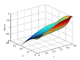
tions for Re = 50 and Re = 500 are obtained at t = 0.625 . Perspective views of u and v for Re = 50 at t = 0.0001 are given in Fig.s 3 and 4.The results given

in Tables 11- 14 demonstrate that the proposed scheme achieves similar results given by [16,20].
Table 1
The numerical results for u in comparison with the exact solu-
(0.5, 0.1) 0.50034 0.50035 0.500003 0.50000
(0.9, 0.1) 0.50000 0.50000 0.500000 0.50000
(0.3, 0.3) 0.54269 0.54332 0.500441 0.50048 (0.7, 0.3) 0.50032 0.50035 0.500003 0.50000 (0.1, 0.5) 0.74215 0.74221 0.555151 0.55568 (0.5, 0.5) 0.54250 0.54332 0.500415 0.50048 (0.9, 0.5) 0.50030 0.50035 0.500014 0.50000 (0.3, 0.7) 0.74212 0.74221 0.554811 0.55568 (0.7, 0.7) 0.54246 0.54332 0.500683 0.50048 (0.1, 0.9) 0.74995 0.74995 0.744215 0.74426

tion at t = 0.5 and t = 2 with

t = 0.0001 ,and Re = 10 .

(0.5, 0.9) 0.74213 0.74221 0.559802 0.55568
(0.9, 0.9) 0.54640 0.54332 0.513409 0.50048
(x, y) t=0.5 t=2

Numerical Exact Numerical Exact

Table 4

The numerical results for v in comparison with the exact solution

at t = 0.5 and t = 2 with

t = 0.0001 , and Re = 100 .

(x, y) t=0.5 t=2

IJSER © 2011 http://www.ijser.org

International Journal of Scientific & Engineering Research Volume 2, Issue 5, May-2011 4

ISSN 2229-5518

Table 5

The numerical results for u in comparison with the exact solution

Table 8

The numerical values for v in comparison with the exact solution

at t = 0.5 and t = 2 with

t = 0.0001 , and Re = 500 .

at t = 0.5 and t = 2 with

t = 0.001 , and Re = 500 .

Table 6

Table 9

The numerical values for u in comparison with the exact solution

The numerical results for v in comparison with the exact solution

at t = 0.5 and t = 2 with

t = 0.01 , and Re = 500 .

at t = 0.5 and t = 2 with

t = 0.0001 , and Re = 500 .

(x, y) t=0.5 t=2
(x, y) t=0.5 t=2

Numerical Exact Numerical Exact

Table 7

Table 10

The numerical values for v in comparison with the exact solution

The numerical values for u in comparison with the exact solution

at t = 0.5 and t = 2 with

t = 0.01 , and Re = 500 .

at t = 0.5 and t = 2 with

t = 0.001 , and Re = 500 .

(x, y) t=0.5 t=2
(x, y) t=0.5 t=2

Numerical Exact Numerical Exact (0.1, 0.1) 0.48732 0.50010 0.49725 0.50000 (0.5, 0.1) 0.50002 0.50000 0.50025 0.50000 (0.9, 0.1) 0.50000 0.50000 0.49932 0.50000 (0.3, 0.3) 0.49531 0.50010 0.50687 0.50000 (0.7, 0.3) 0.50001 0.50000 0.49929 0.50000 (0.1, 0.5) 0.74990 0.75000 0.43945 0.50048 (0.5, 0.5) 0.49438 0.50010 0.49959 0.50000 (0.9, 0.5) 0.49977 0.50000 0.51376 0.50000 (0.3, 0.7) 0.75001 0.75000 0.41654 0.50048 (0.7, 0.7) 0.49324 0.50010 0.51050 0.50000 (0.1, 0.9) 0.75000 0.75000 0.75003 0.75000 (0.5, 0.9) 0.75001 0.75000 0.42895 0.50048 (0.9, 0.9) 0.47380 0.50010 0.56293 0.50000

Numerical Exact Numerical Exact (0.1, 0.1) 1.01286 0.99990 1.00271 1.00000 (0.5, 0.1) 0.99999 1.00000 0.99976 1.00000 (0.9, 0.1) 1.00000 1.00000 1.00066 1.00000 (0.3, 0.3) 1.00481 0.99990 0.99310 1.00000 (0.7, 0.3) 0.99999 1.00000 1.00072 1.00000 (0.1, 0.5) 0.75010 0.75000 1.06061 0.99952 (0.5, 0.5) 1.00571 0.99990 1.00049 1.00000 (0.9, 0.5) 1.00022 1.00000 0.98646 1.00000 (0.3, 0.7) 0.74999 0.75000 1.08353 0.99952 (0.7, 0.7) 1.00676 0.99990 0.98992 1.00000 (0.1, 0.9) 0.75000 0.75000 0.74996 0.75000 (0.5, 0.9) 0.74999 0.75000 1.07091 0.99952 (0.9, 0.9) 1.02725 0.99990 0.93725 1.00000

IJSER © 2011 http://www.ijser.org

International Journal of Scientific & Engineering Research Volume 2, Issue 5, May-2011 5

ISSN 2229-5518

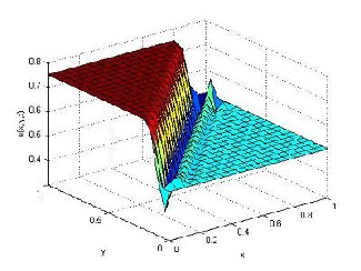
Table 12

Comparison of computed values of v for Re =50 at

t = 0.625

Fig.1.The numerical value of u for Re = 500 at time level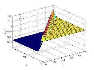

t = 0.5 with

t = 0.001 .

Table 13

Comparison of computed values of u for Re =500 at

t = 0.625 .

Fig.2.The numerical value of v for Re = 500 at time level

Table 14

Table 11

t = 0.5 with

t = 0.001 .

Comparison of computed values of v for Re = 500 at

t = 0.625 .

Comparison of computed values of u for Re = 50 at

t = 0.625 .

IJSER © 2011 http://www.ijser.org

International Journal of Scientific & Engineering Research Volume 2, Issue 5, May-2011 6

ISSN 2229-5518

India, for giving valueable suggestions.
Fig.3.The computed value of u for Re = 50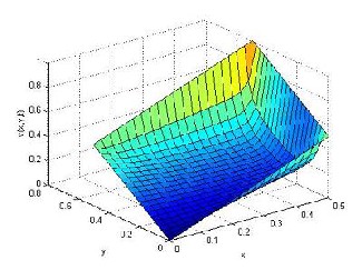

t = 0.625 .

Fig.4.The computed value of v for Re = 50

t = 0.625 .

4 CONCLUSION

at time level
at time level

REFERENCES

[1] Cole JD, “On a quasilinear parabolic equations occurring in aerodynamics,” Quart Appl Math 1951; 9:225-36.

[2] J.D. Logan, ”An introduction to nonlinear partial differential

equations, “ Wily-Interscience, New York, 1994.

[3] L. Debtnath, ”Nonlinear partial differential equations for scien- tist and engineers,” Birkhauser, Boston, 1997.

[4] G. Adomian, ”The diffusion-Brusselator equation,” Comput.

Math. Appl. 29(1995) 1-3.

[5] Bateman H., “some recent researches on the motion of fluids,” Monthly Weather Review 1915; 43:163-170

[6] Burger JM, “A Mathematical Model Illustrating the Theory of

Turbulence, ”Advances in Applied mathematics 1950; 3:201-230 [7] S.K. Chabak, P.K. Sharma, “Numerical simulation of coupled wave equation,” Int Review of Pure and Applied Mathematics

2007; 2(1):59-69.

[8] Hon YC, Mao XZ,”An efficient numerical scheme for Burgers- like equations,”Applied Mathematics and Computation 1998;

95:37-50.

[9] Aksan EN, Ozdes A, ”A numerical solution of Burgers’ equa- tion,”Applied Mathematics and Computation 2004; 156:395-402.

[10] Mickens R, ”Exact solutions to difference equation models of

Burgers’ equation,”Numerical Methods for Partial Differential

Equations 1986; 2(2):123-129.

[11] Kutluay S, Bahadir AR, Ozdes A,”Numerical solution of one- dimensional Burgers’ equation: explicit and exact-explicit finite difference methods,” Journal of Computational and Applied Mathematics 1999; 103:251-261.

[12] Kutluay S, Rsen A,”A linearized numerical scheme for Burgers-

like equations,” Applied Mathematics and Computation 2004;

156:295-305.

[13] Ozis T, Aslan Y,” The semi-approximate approach for solving Burgers’ equation with high Reynolds number,”Applied Ma- thematics and Computation 2005; 163:131-145.

[14] Wenyuan Liao,” An implicit fourth-order compact finite differ-

Crank-Nicolson finite-difference method for two- dimensional coupled nonlinear viscous Burgers’ equa- tions has been presented.The advantage of the proposed method is that it is second order accurate in space and time. The efficiency and numerical accuracy of the present scheme are validated through two numerical ex- amples. The test examples show that the present scheme is unconditionally stable as there is no constraint on time step-size. Numerical results are compared well with those from the exact solutions and previous available results.

ACKNOWLEDGEMENT

The authors are highly grateful to the Vice-chancellor, Dean (FST), The ICFAI University, Dehradun, India, for providing facilities to carry out the present work. The authors would also like to thank Dr. S.K. Chabak, scien- tist, Wadia Institute of Himalayan Geology, Dehradun,

ence scheme for one-dimensional Burgers’ equation,” Applied

Mathematics and Computation 2008; 206:755-764.

[15] C.A.J. Fletcher, “Generating exact solutions of the two- dimensional Burgers’ equation”, Int. J. Numer. Meth. Fluids 3 (1983) 213–216.

[16] P.C. Jain, D.N. Holla, “Numerical solution of coupled Burgers_

equations, “Int. J. Numer. Meth.Eng. 12 (1978) 213–222.

[17] C.A.J. Fletcher,” A comparison of finite element and finite dif- ference of the one- and two-dimensional Burgers’ equations,” J. Comput. Phys., Vol. 51, (1983), 159-188.

[18] F.W. Wubs, E.D. de Goede, “An explicit–implicit method for a

class of time-dependent partial differential equations, “Appl. Numer. Math. 9 (1992) 157–181.

[19] O. Goyon,” Multilevel schemes for solving unsteady equa- tions,” Int. J. Numer. Meth. Fluids 22(1996) 937–959.

[20] Bahadir AR. “A fully implicit finite-difference scheme for two- dimensional Burgers’ equation,” Appl Math Comput 2003;

137:131-7.

IJSER © 2011 http://www.ijser.org

International Journal of Scientific & Engineering Research Volume 2, Issue 5, May-2011 7

ISSN 222S-5518

IJSER 2011 http/fwww l!ser orq