International Journal of Scientific & Engineering Research, Volume 4, Issue 8, August-2013 1289

ISSN 2229-5518

Controller Synthesis:

Case study of an Automated Sun Tracking

System

Ovie E., Nongo S., Adetoro L., Babayo M., Mustapha U. & Agboola O.A.(Ph.D)

Abstract---A major aspect of System dynamics concerns itself with the Modeling, system identification, meas urem ent/obs ervation and control of the system. Such systems could be a single or multi domain systems requiring mixed modeling techniques.

This paper looks at the dynamic model and controller synthesis of a prototype electromechanical system. It

follows a mec hatronics design paradigm and aims to capture as much of the system dynamics as possible.

Two models will be described here for the system in elevation and azimuth. The mathematical models are described and analysis of elevation system’s controller is designed and tested in simulation experiments using Matlab/Simulink. We then present our results with varying controller parameter c onsideration or controller gain tuning.

Index terms: control, gain tuning, mechatronics, mathematical modeling, system identification .

1 INTRODUCTION

System dynamics is a multi-domain[3] discipline requiring the system engineer to understand different engineering domains and their behavior to inputs and corresponding response behavior. For a control system engineer, controller synthesis begins with a proper system model.
Where a proper system model means the system dynamics has been captured with as little simplifying assumptions made during the modeling process.
This paper assumes the modeling has been done to a high degree of accuracy, by utilizing the bond Graph [2][3] method and therefore proceeds to carry out controller synthesis from designing system transfer functions, carrying out open loop tests and then designing a feedback loop for the system in closed loop[1] with the controller in the loop. Fine tuning of the controller is also performed to show the different responses obtainable and how the various gains affect overall system response.
This work follows from dynamic modeling techniques which the author made wide us of during his M.Sc in re- search, specializing in Automatic Control at the French
Grande Ecole, INSA de Lyon with specific theoretical input coming from course work delivered by Bideaux Eric[4].

2 SYSTEM MODEL

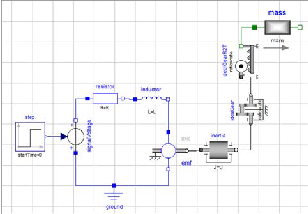
The system model is divided into two active parts. This is because the sun tracker contains two actuators for control in elevation and in Azimuth. The elevation model is first presented here, then the azimuth model.

2.1 Elevation model

International Journal of Scientific & Engineering Research, Volume 4, Issue 8, August-2013 1290

ISSN 2229-5518

With the disturbance term, N(s) set to zero, the final input- output transfer function of the system after substitution is:

𝐺el(𝑠) =

Vsh(s) V1(s) =

5.126s + 5.126

s3 + 2.089s2 + 1.528s + 0.439

2.2 Azimuth model

Figure 1: Elevation equivalent circuit

The Elevation model obtained from the system prototype shown in figure 1 above, yields the following set of first order ODE’s shown below:
The Azimuth model obtained from the system prototype
shown in figure 2 below yields the set of first order ODE’s shown below:

𝑑𝑖1
𝑑𝑡
𝑅1

= −
𝐿1
𝑖1 −

𝑟
𝑛1𝑛2𝑀𝑡𝑜𝑡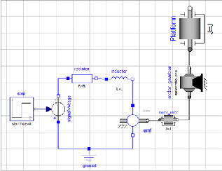

𝑣𝑠ℎ + 𝑉1
𝑑𝑣𝑠ℎ = − 𝑟
𝑖1 − 𝑘2𝑣
𝑚𝑔𝑛3

+

𝑑𝑡
𝑛1𝑛2𝑘1𝐿1

𝑠ℎ

𝑘1
And in equivalent state space representation x = Ax+Bu we
have :

Figure 2: Azimuth equivalent circuit

� 𝚤1 � = �

𝑅1

−

𝐿1

𝑟1

𝑛1𝑛2𝑀𝑡𝑜𝑡� � 𝑖1 � + �𝑣1� 𝑢

𝑣𝑠ℎ

𝑟1

−

𝑛1𝑛2𝑅1𝐿1

−𝑘2

𝑣𝑠ℎ 𝑛

𝑑𝑖2 𝑅2 𝑟

= − 𝑖2 −
𝑤2 + 𝑉2
Where k1, k2 are constants grouping some parameters
𝑑𝑡
𝑑𝑤2

= −
𝑑𝑡

𝑟
𝐿2
𝐿2
𝑖2 −
𝐽𝑟2
𝑟𝑟

𝑤2 +
𝐽𝑟2

𝑟𝑟
𝐽_𝑝𝑙
𝑤_𝑝𝑙
defined by:
𝑑𝑤_𝑝𝑙

=
𝑑𝑡

𝑟𝑟
𝐽𝑟2
𝑤2 −

𝑟𝑟
𝐽_𝑝𝑙
𝑤_𝑝𝑙
This model takes for its input v1 and gives a response
which is equivalent to the shaft velocity Vsh. After transforming the first order ODE’s, the resulting transfer function of the elevation system which links these two variables evaluates to:
With equivalent state space representation given as:

𝑘3𝑘4𝐿1 L1

𝑅2 𝑟

�𝑠 +

𝑠𝐿1 + 𝑅1

+ 𝑘2� 𝑉𝑠ℎ(𝑠) = k4

sL1 + R1

V1(s) + N(s)

− − 0

⎛ 𝐿2 𝐽𝑟2 ⎞

𝑣2

𝚤2

⎜– 𝑟

𝐹𝑟𝑟

−

𝐹𝑟𝑟 ⎟

𝑖2 0

� 𝑤2 � = ⎜

𝐿2

𝐽𝑟2

𝐽𝑝𝑙

⎟ � 𝑤2 � + �

� 𝑢

Where N(s) is a disturbance term which is due to the mass

𝑤𝑝𝑙 ⎜ 0

⎝

𝐹 𝑟𝑟

𝐽𝑟2

− 𝐹𝑟𝑟 ⎟

𝐽𝑝𝑙

⎠

𝑤𝑝𝑙 0

hanging down while the panel load is at a maximum incline to the vertical. K3=r/(n1n2Mtot) and k4 = r/(n1n2k1L1).
The azimuth model takes v2 as its input and the response is observed on the platform’s angular velocity Wpl. After making necessary substitutions for the overall Azimuth

International Journal of Scientific & Engineering Research, Volume 4, Issue 8, August-2013 1291

ISSN 2229-5518

transfer function, the following form is obtained for the system transfer function in open loop:

𝐺az(𝑠) =

Wpl(s) V2(s)

3.1 Elevation dynamic parameters

Relating the output platform angular velocity to the input
supply voltage, the transfer function for the azimuth
dynamics is obtained but not shown here for lack of space
It must be noted that, this coarse form of the azimuth transfer function made little or no simplifications to the
Azimuth model obtained from the system dynamic studies. The parameters specified in this equation are:
K1= r2/j2, k2=Frr/Jr2, k3= Frr/Jpl with electric time constant
τ2=L2/R2
As a first approximation before system identification, all the constants are set to unity for open loop test and analysis. This generates a system transfer function which is strictly proper( having the degree of the transfer function characteristic polynomial’s denominator greater than degree of numerator)

s3 + 3s2 + 2s

𝐺az(𝑠) =

s6 + 4s5 + 9s4 + 16s3 + 19s2 + 12s + 3

A resume of the identified elevation dynamic parameters is given below in Table 1:

Table 1: Open loop Elevation identification parameters

Parameters	Ziegler-Nichols	Broida
τ	0.0	2.365
response time (T)	0.0	1.741

Employing Ziegler-Nichols method, where t1 is time at 28% of max. response and t2 is time at 40% of max. response. The open loop response gives a Time delay of about 0.1 seconds. The time constant(63% of output response) for the system in open loop is 3.89sec.
A Matlab/simulink model for the elevation dynamics was used to obtain the open loop response shown in figure 3 the closed loop response of the system is obtained from the signal block diagram given by figure 4, with the response for the closed loop system shown in figure 7 below:

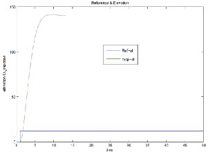
3 MODELING AND SYSTEM IDENTIFICATION

The system identification for the elevation dynamic follows from the method of Ziegler-Nichols and Broida[1]. From the response curve seen in figure 3, the system is approximately a first order system. Using Broida parameters, the system response time (T) and time constant is calculated following the formulas given below:

𝑇 = 2.8 ∗ 𝑡1 − 1.8 ∗ 𝑡2

𝜏 = 5.5 ∗ (𝑡2 − 𝑡1)

Open loop analysis was carried out on both elevation and azimuth models obtained previously in the analog or
continuous domain. We then proceed to identify the system parameters which have utility in synthesizing a suitable controller for each subsystem taking into consideration the system dynamics involved.

Figure 3: elevation open loop response

International Journal of Scientific & Engineering Research, Volume 4, Issue 8, August-2013 1292

ISSN 2229-5518

τ	0.0	1.7626
response time (T)	0.0	1.1165

4 MODELING AND CONTROLLER SYNTHESIS

Figure 4: closed loop elevation diagram showing feedback

3.2 Azimuth dynamic parameters

Similarly, for the azimuth dynamics we obtain the open loop response shown in figure 5 as obtained from simulation experiments in open loop, while the resume of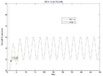

the identified azimuth parameters is given in Table 2 below:

Figure 5: Open loop Azimuth response

Table 2: Open loop Azimuth identification parameters

Parameters Ziegler-Nichols Broida
Since the elevation response follows a first order system
response curve, a PI controller is chosen with gains tuned following the Chiens-Hrones-Reswick formulas in tracking mode [1].
From the open loop analysis, the elevation controller synthesis follows
Kp=0.35x T/τ = 0.257 &
Ti=1.2xT=2.089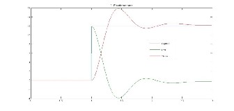

from where the closed loop control response is shown below:

Figure 6: Closed loop elevation response

The azimuth controller synthesis follows
Kp=0.35x T/τ =0.222 &
Ti=1.2xT=1.3398

4.1 Closed loop system

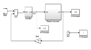
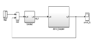
After controller synthesis, the controller is incorporated into the system with the resulting system diagram shown in figure 6 below:

International Journal of Scientific & Engineering Research, Volume 4, Issue 8, August-2013 1293

ISSN 2229-5518

With the constants defined as:

Figure 7: Azimuth closed loop block schematic

4.2 Stability analysis

Various methods exist to test the stability of dynamic systems such as that describing the elevation model of the sun tracker. Some widely used methods are:
• Routh- Hurwitz criterion
• Eigenvalue analysis
• Lyapunov method and LaSalle's invariance
principle
• Small or short time stability analysis

4.3 Stability determination using Eigenvalue analysis

To perform stability analysis on the elevation system, the closed loop response will have to be made use of. Recalling
the form of the transfer function in open loop for the elevation subsystem given by equation 3; we can
Incorporate the behavior of the PID controller recalling that the new input from the PID controller is given by:

𝐾𝑖
𝑈(𝑠) = 𝐾𝑝 �1 + 𝑠 + 𝑠𝐾𝑑� 𝐸(𝑠)
with U(s) substituting Vin in equation 3 and the error term
from feedback action E(s) being replaced by Vd(s)-Vsh(s), we will have a new closed loop transfer function given by:
K1*=k4kpkdL1
K2*=k4kpL1
K3*=k4kpkiL1
K4*=L1
K5*=R1+k2L1+k4kpkdL1
K6*=k2R1+k3k4L1+k4kpL1
K7*=k4kpkiL1
Stability of the system can be inferred from the poles of the TF denominator. Since all the eigenvalues will be real and strictly negative, the system is eigenvalue stable as all its characteristic poles will be found on the left half of the complex plane.

4.4 Stability analysis using Exponential time growth

The stability analysis looks at the dynamics of the system in exponential time. If the error of the system decays to zero as time goes to infinity then the system is said to be stable. This is seen from the plot given in figure 7 of the closed loop dynamic controller response of the elevation system studied.

5 EXPERIMENTAL RESULTS AND ANALYSIS

Experiments were carried out in simulation and the results are shown here with utilized parameters. The system is controllable using a simple PID controller with gain tuning
as shown in figure 6 with various tuned values for controller gains. From the open loop response of the elevation system, we see that divergence from the nominal step input occurs. The voltage equivalent for this response means a sharp rise in input voltage to the elevation motor which is not supposed to be. The controller addresses this situation by forcing the output to be within the desired response of 12 volt.
The azimuth open loop response shows a wide divergence in the motor behavior. This is seen through the strong

𝐺elcl(𝑠) =

Vsh(s) Vd(s) =

s2K1∗ + sK2∗ + K3∗

s3 K4∗ + s2 K5∗ + sK6 + K7∗

oscillatory response observed. Using a simple PID might

International Journal of Scientific & Engineering Research, Volume 4, Issue 8, August-2013 1294

ISSN 2229-5518

not be ideal for the control of this system and ongoing tests are in place to resolve the issue of the azimuth control.

6 DISCUSSION AND CONCLUSION

The modeling, analysis and control of the sun tracker
system are looked at from a control system stand point with
some results of the performed experiments given. Gain tuning is employed to adjust the system response to within the desired values.
While standard methods[1] exist and are used to compute the start gain parameters for the controller, it is seen that working gain values could widely diverge from the calculated or nominal as was the case with this work. This is being attributed to the unknown system dynamics ignored as part of this analysis as the parts used were sourced for locally in the market without a thorough knowledge of the internal components especially as it concerns frictional effects, reduction gear ratios and other unaccounted for parameters which could play a role in this divergence.
In summarizing, the goal of building a system model and carrying out analysis needed for controller synthesis was achieved through this paper with the dissemination of such knowledge to interested scientists and engineers.
Further work will be to carry out detailed numerical simulations to gain further insight into the system behavior.
References
[1] K. Hamiti, A. Voda-Besanqon and H. Roux-Buisson, POSITION CONTROL OF A PNEUMATIC ACTUATOR UNDER THE INFLUENCE OF STICTION. UJFG-LIME, B.P. 53, 38041 Grenoble Cedex, France, Laboratoire d’Automatique de Grenoble, ENSIEG, B.P.
46,
38402 Saint Martin d’Heres, France,
1996.
[2] Henry M. Paynter
An Epistemic Prehistory of Bond Graphs
Elsevier’s Press,
2000.
[3] Karnoop, Rosenberg & Margolis
Modeling, Simulation and Control of Dynamic systems
Elsevier’s Press,
2011.
[4] Bideaux Eric
Modeling, Simulation and Control of Dynamic systems
INSA de Lyons, France
2012.
[5] Ovie, E., Bond Graph approach to Dynamic system
Modeling, NASRDA, Abuja. March, 2013.
[6] Lamport, L., LaTeX : A Documentation Preparation
System User’s Guide and Reference Manual,
Addison-Wesley Pub Co., 2nd edition, August
1994.