International Journal of Scientific & Engineering Research Volume 4, Issue 2, February-2013 1

ISSN 2229-5518

Comparative study of Grillage method and Finite

Element Method of RCC Bridge Deck

R.Shreedhar, Rashmi Kharde

Abstract- The simplest form of bridge is the single-span beam or slab which is simply supported at its ends. Many methods are used in analyzing bridges such as grillage and finite element methods. Since its publication in 1976 up to the present day, Edmund Hambly’s book “Bridge Deck Behaviors” has remained a valuable reference for bridge engineers. During this period the processing power and storage capacity of computers has increased by a factor of over 1000 and analysis software has improved greatly in sophistication and ease of use. In spite of the increase in computing power, bridge deck analysis methods have not changed to the same extent, and grillage analysis remains the standard procedure for most bridges deck. The grillage analogy method for analyzing bridge superstructures has been in use for quite some time. An attempt is made in this paper to provide guidance on grillage idealization of the structure, together with the relevant background information. Guidance is provided on the mesh layout. The bridge deck is analyzed by both grillage analogy as well as by finite element method. Bridge deck analysis by grillage method is also compared for normal meshing, coarse meshing and fine meshing. Though finite element method gives lesser values for bending moment in deck as compared to grillage analysis, the later method seems to be easy to use and comprehend.

——————————  ————————

1. INTRODUCTION

Many methods are used in analyzing bridges such as grillage and finite element methods. Generally, grillage analysis is the most common method used in bridge analysis. In this method the deck is represented by an equivalent grillage of beams. The finer grillage mesh, provide more accurate results. It was found that the results obtained from grillage analysis compared with experiments and more rigorous methods are accurate enough for design purposes. If the load is concentrated on an area which is much smaller than the grillage mesh, the concentration of moments and torque cannot be given by this method and the influence charts described in Puncher can be used. The orientation of the longitudinal members should be always parallel to the free edges while the orientation of transverse members can be either parallel to the supports or orthogonal to the longitudinal beams. The other method used in modelling the bridges is the finite element method. The finite element method is a well known tool for the
————————————————

1. Prof. R. Shreedhar is Associate Professor in the Department of Civil Engineering in Gogte Institute of Technology Belgaum (Karnataka), INDIA, PH:+919845005722.

E-mail: rshree2006@gmail.com

2. Rashmi Kharde is currently pursuing master degree in Structural

Engineering at Gogte Institute of Technology Belgaum

(Karnataka), INDIA, PH: +918904836980.

E-mail: rashmikharde7@gmail.com
solution of complicated structural engineering problems, as it is capable of accommodating many complexities in the solution. In this method, the actual continuum is replaced by an equivalent idealized structure composed of discrete elements, referred to as finite elements, connected together at a number of nodes.

2. SLAB DECK

The simplest form of bridge is the single-span beam or slab which is simply supported at its ends. This form is widely used when the bridge crosses a minor road or small river. In such cases, the span is relatively small and multiple spans are infeasible and/or unnecessary. The simply supported bridge is relatively simple to analyze and to construct but is disadvantaged by having bearings and joints at both ends. The cross-section is often solid rectangular but can be of any of the forms presented above. A bridge deck can be considered to behave as a beam when its length exceed its width by such an amount that when loads cause it to bend and twist along its length, its cross-sections displace bodily and do not change shape. Many long-span bridges behave as a beam because the dominant load is concentric so that the direction of the cross- section under eccentric loads has relatively little influence on the principle bending stresses [Edmund, 1991].

IJSER © 2013 http://www.ijser.org

International Journal of Scientific & Engineering Research Volume 4, Issue 2, February-2013 2

ISSN 2229-5518

3. LOADS ON BRIDGES

3.1 DEAD LOAD

The deck of the bridge subjected to dead loads comprising of its self weights due to wearing coat, parapet, kerb etc. which are permanently stationary nature. The dead load act on the deck in the form of the distributed load. These dead loads are customarily considered to be done by the longitudinal grid members only giving rise to the distributed loads on them. The distributed load on the longitudinal grid member is idealized into equivalent nodal loads. This is specially required to be done when the distributed load is non uniform. On the other hand, if the self load is uniform all along the length of longitudinal grid line then it is not necessary to find the equivalent nodal load and instead it can be handled as a uniformly distributed load (udl) itself. Further, if the dead load is udl but its center is not coincident with the longitudinal grid
line then it is substituted by a vertical udl.
transferred to the surrounding nodes of the panels to facilitate the analysis.
In order to obtain the maximum response resultants for the design, different positions of each type of loading system are to be tried on the bridge deck. For this purpose, the wheel loads of a vehicular loading system are placed on the bridge and moved longitudinally and transversely in small steps of occupy a large number of different positions on the deck. The largest force response is obtained at each node discrete element, referred to as finite elements
,connected together at a number nodes.


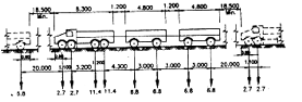
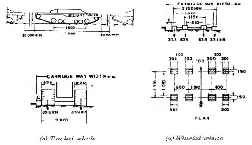
Figure 1, IRC Class A loading

3.2 LIVE LOAD

The main live loading on highway bridges is of the vehicles moving on it. Indian Roads Congress (IRC) recommends different types of standard hypothetical vehicular loading systems, for which a bridge is to be designed.
The vehicular live loads consist of a set of wheel loads. These are distributed over small areas of contacts of wheels and form patch loads. These patch loads are treated as concentrated loads acting at the centre of contact areas. This is a conservative assumption and is made to facilitate the analysis. The effect of this assumption on the result is very
small and does not make any appreciable change in the design.

3.3. IMPACT LOAD

Figure 2, IRC AA loading
IRC Class A two lane, Class AA Tracked and Wheeled, Class 70R Tracked and Wheeled loads are shown in Figs. Three different wheel arrangements for Class 70R Wheeled loads are in existence Class 70R Tracked load may be idealized into 20 point loads of 3.5tonns each, 10 point loads on each track. The total load of the vehicle in this case is 70 tonnes.
One Class A or Class B loading can be adopted for every lane of the carriageway of the bridge. Thus, for a two- lane bridge, we can have two lanes of Class A or Class B loading. However, for all other vehicles, only one vehicle loading per two lanes of the carriageway is assumed. It is assumed in the design that the vehicles can not go closer to the kerb by certain recommended clear distance.
The Wheel loads of the vehicle will be either in the panes formed by the longitudinal and transverse grid lines, of
on the nodes. The wheel loads falling in the panels are to be
Another major loading on the bridge superstructure is due to the vibrations caused when the vehicle is moving over the bridge. This is considered through impact loading. IRC gives impact load as a percentage of live load. As per IRC code, impact load varies with type of live loading, span length of bridge and whether it is a steel or a concrete bridge. The impact load, so evaluated, is directly added to the corresponding live load.The dynamic effect caused due to vertical oscillation and periodical shifting of the live load from one wheel to another when the locomotive is moving is known as impact load. The impact load is determined as a product of impact factor, I, and the live load. The impact factors are specified by different authorities for different types of bridges.
The impact factors to be considered for different classes of I.R.C. loading as follows:

IJSER © 2013 http://www.ijser.org

International Journal of Scientific & Engineering Research Volume 4, Issue 2, February-2013 3

ISSN 2229-5518

a) For I.R.C. class A loading

The impact allowance is expressed as a fraction of the applied live load and is computed by the expression,
I=A/ (B+L)
Where, I=impact factor fraction
A=constant having a value of 4.5 for a reinforced concrete bridges and 9.0 for steel bridges.
B=constant having a value of 6.0 for a reinforced concrete bridges and 13.5 for steel bridges.
L=span in meters.
For span less than 3 meters, the impact factor is 0.5 for a reinforced concrete bridges and 0.545 for steel bridges. When the span exceeds 45 meters, the impact factor is 0.088 for a reinforced concrete bridges and
0.154 for steel bridges.

b) For I.R.C. Class AA or 70R loading

3. For span less than 9 meters
1) For tracked vehicle- 25% for a span up to 5m linearly reduced to a 10% for a span of 9m.
2) For wheeled vehicles-25%
4. For span of 9 m or more
1) For tracked vehicle- for R.C. bridges, 10% up to a span of 40m. For steel bridges, 10% for all spans.

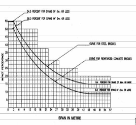
2) For wheeled vehicles- for R.C. bridges, 25% up to a span of 12m. For steel bridges, 25% for span up to 23 meters.

4. EFFECTIVE WIDTH METHOD

This method is applicable where one way action prevails. For this the slab needs to be supported on only two edges, however very long slab may be supported on all the four edges. this method based on the observation that it is not only the strip of the slab immediately below the load that participates in taking the load prevails is known as the effective width of dispersion. The extent of effective width depends on the location of the wheel load with reference to support and dimensions of the slab. Thus, the concentrated load virtually transforms into a uniformly distributed load, distributed along some length (dispersed length along the span) and width.

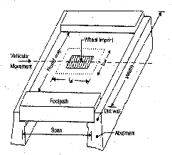
Figure 4: Load dispersion on slab

4.1EFFECTIVE WIDTH OF DISPERSION

For the slab supported on two edges and carrying concentrated loads, the maximum live load bending moment is calculated by considering the effective width of the slab. This effective width also called the effective width of dispersion is measured parallel to the supporting edge of the span. Bridge deck slab have to be designed for I.R.C. loads, specified as class AA or A depending on the importance of the bridge. for slab supported on two opposite sides, the maximum bending moment caused by a wheel load may be assumed to be resisted by an effective width of the slab measured parallel to the supporting edges.
For a single concentrated load the effective width of the dispersion may be calculated by the equation,

be= K x (1-x/L) + bw

Figure 3 Impact percentage for highway bridges
where,
be= Effective width of slab on which the load acts

IJSER © 2013 http://www.ijser.org

International Journal of Scientific & Engineering Research Volume 4, Issue 2, February-2013 4

ISSN 2229-5518

L= Effective span
X= distance of center of gravity of load from nearer support
Bw=breadth of concentration area of load,i.e. width of dispersion area of the wheel load on the slab through the wearing coat.
This is given by (w + 2h), where h is the thickness of the wearing coat, w is the contact width of the wheel on the slab perpendicular to the direction of movement.
K= a constant depending on the ratio (B/L) where ’B’
is the width of the slab.
The values of the constant ‘K’ for different values of ratio (B/L ) is compiled in Table 1 for simply supported and continuous slabs.

Table 1 Values of K (I.R.C. 6-2000, sec2)

It is obvious that the maximum value of the effective width will be equal to the width of the slab. For two or more concentrated loads in a line, in the direction of the span, the net effective width should be calculated. A closer view of this width along the span and across span is shown in fig 5.

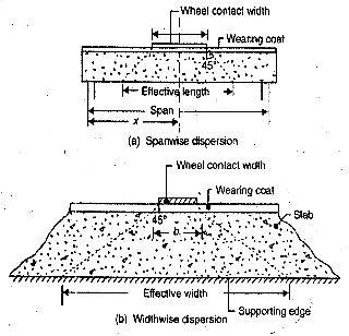
Figure 5 Load Dispersion

4.2 DISPERSION LENGTH

Dispersion of the wheel load along the span is known as the effective length of dispersion. It is also called the dispersion length.
It can be calculated as shown below:
Dispersion length = length of the tyre contact + (2 X overall thickness of the deck including the thickness of wearing coat)

5. FINITE ELEMENT ANALYSIS

Finite elements, referred to as finite elements, connected together at a number of nodes. The finite elements method was first applied to problems of plane stress, using triangular and rectangular element. The method has since been extended and we can now use triangular and rectangular elements in plate bending, tetrahedron and hexahedron in three-dimensional stress analysis, and curved elements in singly or doubly curved shell problems. Thus the finite element method may be seen to be very general in application and it is sometimes the only valid analysis for the technique for solution of complicated structural engineering problems. It most accurately predicted the bridge behavior under the truck axle loading.
The finite element method involves subdividing the actual structure into a suitable number of sub-regions that are called finite elements. These elements can be in the form of line elements, two dimensional elements and three-dimensional

IJSER © 2013 http://www.ijser.org

International Journal of Scientific & Engineering Research Volume 4, Issue 2, February-2013 5

ISSN 2229-5518

elements to represent the structure. The intersections between the elements are called nodal points in one dimensional problem where in two and three-dimensional problems are called nodal line and nodal planes respectively. At the nodes, degrees of freedom (which are usually in the form of the nodal displacement and or their derivatives, stresses, or combinations of these) are assigned. Models which use displacements are called displacement models and some models use stresses defined at the nodal points as unknown. Models based on stresses are called force or equilibrium models, while those based on combinations of both displacements and stresses are termed mixed models or hybrid models.
Displacements are the most commonly used nodal variable, with most general purpose programs limiting their nodal degree of freedom to just displacements. A number of displacement functions such as polynomials and trigonometric series can be assumed, especially polynomials because of the ease and simplification they provide in the finite element formulation.
Finite element needs more time and efforts in modeling than the grillage. The results obtained from the finite element method depend on the mesh size but by using optimization of the mesh the results of this method are considered more accurate than grillage. The finite element method is a well-known tool for the solution of complicated structural engineering problems, as it is capable of accommodating many complexities in the solution. In this method, the actual continuum is replaced by an equivalent idealized structure composed of discrete elements, referred to as finite elements, connected together at a number of nodes.
The availability of sophisticated computers over the last three decades has enabled engineers to take up challenging tasks and solve intractable problems of earlier years. Nowadays rapid decrease in hardware cost has enabled every engineering firm to use a desk top computer or micro processor. Moreover they are ideal for engineering design because they easily provide an immediate access and do not have the system jargon associated with large computer system. It is to be expected that software to be sold or leased and the hardware supplied with software. After the initial phase, where only principles of gravity and statics were enunciated resulting in ambiguity in applying to structural problem, Mathematicians took over from around 1400 A. D. and presented a variety of formulations and solutions. Purely, as
exercise in basic science, around 1700A.D. these formulations
and solutions found practical significance in applications to structures with proper approximations and adaptations. New methods exclusive for structural analysis were evolved like slope deflection, moment distribution and relaxation. Later part of this period witnessed the emergence of superfast calculation and later computers. Thus started the era of computers wherein the developments in structural analysis and design were and are still complementary to those in computers. A reorientation to the developments and formulation proposed in the earlier eras took place mainly to use the advantageous features of computers like high speed arithmetic, large information storage and limited logic, bringing in matrix methods of analysis and later finite element and boundary integral element methods.
In recent years, the increasing availability of high speed computers have caused civil engineers to embrace finite element analysis as a feasible method to solve complex engineering problems. It is common for personal computers for home use today are more powerful than supercomputer previous years. Therefore, the increasing popularity of Finite Element Analysis can be attributed to the advancement of computer technology.

6. GRILLAGE ANALYSIS

This method of analysis using grillage analogy, based on stiffness matrix approach, was made amenable to computer programming by Lightfoot and Sawko. West made recommendations backed by carefully conducted experiments on the use of grillage analogy. He made suggestions towards geometrical layout of grillage beams to simulate a variety of concrete slab and pseudo-slab bridge decks, with illustrations. Gibb developed a general computer program for grillage analysis of bridge decks using direct stiffness approach that takes into account the shear deformation also, Martin then followed by Sawko derived stiffness matrix for curved beams and proclaimed a computer program for a grillage for the analysis of decks, curved in plan. For any given deck, there will invariably be a choice amongst a number of methods of analysis which will give acceptable results. When the complete field of slab, pseudo-slab and slab on girders decks are considered, grillage analogy seems to be completely universal with the exception of Finite Element and Finite Strip methods which will always be cost wise heavy for a structure as simple as a slab bridge. Further, the rigorous methods of analysis like Finite Element Method, even today, are considered too

IJSER © 2013 http://www.ijser.org

International Journal of Scientific & Engineering Research Volume 4, Issue 2, February-2013 6

ISSN 2229-5518

complex by some bridge designers. Space frame idealization of bridge decks has also found favour with bridge designers. The idealization is particularly useful for a box girder structure with variable width r depth where the finite strip and folded plate techniques are inappropriate. However, Scordelis concluded certain disadvantages of space frame analysis to the extent that the computer time involved is excessive while the solution is still approximate. The grillage analogy method can be applied to the bridge decks exhibiting complicated features such as heavy skew, edge stiffening, deep haunches over supports, continuous and isolated supports, etc., with ease. The method is versatile, in that, the contributions of kerb beams and footpaths and the effect of differential sinking of girders ends over yielding supports such as in the case of neoprene bearings, can be taken into account. Further, it is easy for an engineer to visualize and prepare the data for a grillage. Also, the grillage analysis programs are more generally available and can be run on personal computers. The method has proved to be reliably accurate for a wide variety of bridge decks.
The method consists of converting the bridge deck structure into a network of rigidly connected beams or into a network of skeletal members rigidly connected to each other at discrete nodes i.e. idealizing the bridge by an equivalent grillage. The deformations at the two ends of a beam element are related to a bending and torsional moments through their bending and torsion stiffness. The load deformation relationship at the two ends of a skeletal element with reference to the member axis is expressed in terms of its stiffness property. This relationship which is expressed with reference to the member co-ordinate axis, is then transferred to the structure or global axis using transformation matrix, so that the equilibrium condition that exists at each node in the structure can be satisfied.The moments are written in terms of the end-deformations employing slope deflection and torsional rotation moment equations. The shear force in the beam is also related to the bending moment at the two ends of the beam and can again be written in terms of the end deformations of the beam. The shear and moment in all the beam elements meeting they a node and fixed end reactions, if any, at the node, are summed up and three basic statical equilibrium equations at each node namely ΣFZ = 0, ΣMz= 0 and ΣMy= 0 are
satisfied. The bridge structure is very stiff in the horizontal
plane due to the presence of decking slab. The transitional displacements along the two horizontal axes and rotation about the vertical axis will be negligible and may be ignored in
the analysis. Thus a skeletal structure will have three degrees of freedom at each node i.e. freedom of vertical displacement and freedom of rotations about two mutually perpendicular axes in the horizontal plane. In general, a grillage with n nodes will have 3n degrees of freedom or 3n nodal deformations and
3n equilibrium equations relating to these. All span loading are converted into equivalent nodal loads by computing the fixed end forces and transferring them to global axes. A set of simultaneous equations are obtained in the process and their solutions result in the evaluation of the nodal displacements in the structure. The member forces including the bending the torsional moments can then be determined by back substitution in the slope deflection and torsional rotation moment equations. Bridges are frequently designed with their decks skew to the supports, tapered or curved in plan. The behaviour and rigorous analysis are significantly complicated by the shapes and support conditions but their effects on grillage analysis are of inconvenience rather than theoretical complexity. Most road bridges of beams and slab construction can be analyzed as three dimensional structure by a space frame analysis which is an extension of grillage analogy. The mesh of the space frame in plan is identical to the grillage, but various transverse and longitudinal members are placed coincident with the line of the centroids of the downstand or upstand members they represent. For this reason, the space frame is sometimes referred to as downstand Grillage. The longitudinal and transverse members are joined by vertical members, which being short are very stiff in bending. The downstand grillage behaves in a similar fashion as the plane grillage under actions of transverse and longitudinal torsion and bending in a vertical plane and consequently, sectional properties of these are calculated in the same way. When a bridge deck is analyzed by the method of Grillage Analogy, there are essentially five steps to be followed for obtaining design responses :

 Idealization of physical deck into equivalent grillage

 Evaluation of equivalent elastic inertia of members of grillage

 Application and transfer of loads to various nodes of grillage

 Determination of force responses and design envelopes and

 Interpretation of results.

IJSER © 2013 http://www.ijser.org

International Journal of Scientific & Engineering Research Volume 4, Issue 2, February-2013 7

ISSN 2229-5518

6.1 GENERAL GUIDELINES FOR GRILLAGE LAYOUT

6.1.1 IDEALIZATION OF DECK INTO EQUIVALENT GRILLAGE

Because of the enormous variety of deck shapes and support conditions, it is difficult to adopt hard and fast rules for choosing a grillage layout of the actual structure However, some basic guidelines regarding the location, direction, number, spacing etc. of the longitudinal and transverse grid lines forming the idealized grillage mesh are followed in the deck analysis. But each type of deck has its own special features and need some particular arrangements for setting idealized grid line.

6.1.2 LOCATION AND DIRECTION OF GRID LINES :Grid lines are to be adopted along lines of strength. In the longitudinal direction, these are usually along the centre line of girders, longitudinal webs, or edge beams, wherever these are present. Where isolated bearings are adopted, the grid lines are also to be chosen along the lines joining the centres of bearings. In the transverse direction, the grid lines are to be adopted, one at each end connecting the centres of bearings and along the centre lines of transverse beams, wherever these exits.In general, the grid lines should coincide with the centre of gravity of the sections but some shift or deviation is permissible, if this simplifies the grid layout or if it assigns more clearly and easily the sectional properties of the grid members in the other direction.

6.1.3 NUMBER AND SPACING OF GRID LINES Wherever possible, an odd number of longitudinal and transverse grid lines are to be adopted. The minimum number of longitudinal grid lines may be three and the minimum number of transverse grid lines per span may be five. The ratio of spacing of transverse grid lines of those of longitudinal grid lines may be chosen between 1.0 and 2.0. This ratio usually reflects the span to width ratio of the bridge. Thus, for a short span and wide bridge, it should be close to 1.0 and for long span and narrow bridge, this ratio may be kept closer to 2.0.Gridlines are usually uniformly placed, but their spacing can be varied, if required, depending upon the situation. For example, closer transverse grid lines should be adopted near a continuous support as the longitudinal moment gradient is steep at such locations.It may be noted that in the grillage analysis, an increase in number of grid lines consequently increases the accuracy of computation, but the effort involved is also more and soon it becomes a case of diminishing return. In a

continuous girder bridge, more than one longitudinal physical
beam can be represented by one grid line. For slab bridges, the grid lines need not be closer than two to three times the depth of slab.Following points give a summary of the guidelines to convert an actual bridge deck into a grid for grillage analysis :

 Grid lines are placed along the centre line of the existing beams, if any and along the centre line of left over slab, as in the case of T-girder decking.

 Longitudinal grid lines at either edge be placed at

0.3D from the edge for slab bridges, where D is the depth of the deck.

 Grid lines should be placed along lines joining bearings.

 A minimum of five grid lines are generally adopted in each direction.

 Grid lines are ordinarily taken at right angles.

 Grid lines in general should coincide with the CG of the section. Some shift, if it simplifies the idealisation, can be made.

 Over continuous supports, closer transverse grids may be adopted. This is so because the change is more depending upon the bending moment profile.

 For better results, the side ratios i.e. the ratio of the grid spacing in the longitudinal and transverse directions should preferably lie between 1.0 to 2.0.

7. DESIGN EXAMPLE

A. BY GRILLAGE ANALYSIS

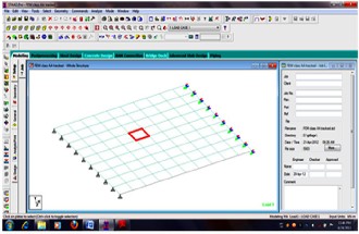
A two lane right slab bridge is chosen for the example with the clear span of 9m. The equivalent grid is shown in fig.6 and is referred to as normal mesh. It consists of seven longitudinal and seven transverse grid lines. The bridge is analyzed for 2 different types of IRC live loadings along with corresponding impact factors. The IRC live loading chosen are;
i) Class AA Tracked. ii) Class A loading.
These loadings are moved on the bridge in a suitably chosen interval both longitudinally and transversely so that the load transverses the entire length and width of the deck. For this example the interval of 500mm has been chosen for longitudinal movements of all types of loadings. In transverse direction the intervals are so chosen that the load transverses the full deck width in 5 or 6 steps.

IJSER © 2013 http://www.ijser.org

International Journal of Scientific & Engineering Research Volume 4, Issue 2, February-2013 8

ISSN 2229-5518

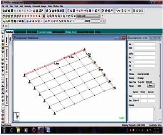
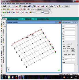
Figure 6 : Normal grid mesh
This example is further used to study the effect of size of the mesh formed by the grid lines fig.7 shows a courser mesh of the same bridge where the numbers of longitudinal grid lines have been reduced from 7 to 5 but the numbers of transverse grid lines have been kept the same fig.8 shows a finer mesh for the same bridge where the number of transverse grid lines have been increased from 7 to 11 but the number of longitudinal grid lines are kept the same two types of IRC live loading as above keeping the longitudinal and transverse intervals for the various IRC loadings same in the analysis of grid of figure.

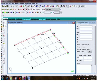
Figure 7: Course grid mesh
Figure 8: Fine grid mesh

Table 2: Maximum longitudinal bending moments and maximum shear force

The variation of course grid compared to normal grid = 1.26% The variation of fine grid compared to normal grid = 0.99%
This shows that some variations in fineness or coarseness in mesh pattern can be adopted if desired without affecting the accuracy in any significant manner.

IJSER © 2013 http://www.ijser.org

International Journal of Scientific & Engineering Research Volume 4, Issue 2, February-2013 9

ISSN 2229-5518

B. BY FINITE ELEMENT ANALYSIS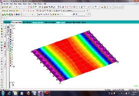

Figure 11 Bending moment (class AA-tracked)

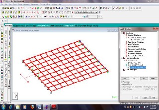
Figure 8 FEM model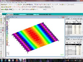
Figure 12 Bending moment (class A)

Table 3 Maximum longitudinal bending moments

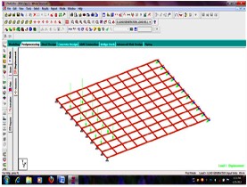
Figure 9 Live load (class AA-Tracked)

CONCLUSION

Figure 10 Live load (class A)
The focus of this modelling is to find the reason of the results differences of the two models (Grillage, Finite Element), while the objective is to simulate the behaviour of bridge structure in terms of bending moment value. AThe modeling
and analysis is done by Staad-Pro software.

IJSER © 2013 http://www.ijser.org

International Journal of Scientific & Engineering Research Volume 4, Issue 2, February-2013 10

ISSN 2229-5518

In general for practical slab bridge deck, result for finite element gives lesser value in terms of bending moment compared with grillage model. Therefore it can be concluded that analysis by using finite element method gives more economical design when compared with the grillage analysis. But the benefit for grillage analysis is that it is easy to use and comprehend.

ACKNOWLEDGMENT

The authors thank the Principal and Management of KLS Gogte Institute of Technology, Belgaum for the continued support and cooperation in carrying out this study

REFERENCES

[1] “Bridge Design using the STAAD.Pro/Beava”, IEG Group, Bentley Systems, Bentley Systems Inc., March 2008.

[2] “Bridge Deck Analysis” by Eugene J O’Brein and Damien and L Keogh.

[3] “ Bridge Deck Behaviour” by Edmund Hambly

[4] “Grillage Analogy in Bridge Deck Analysis” by C.S.Surana and

R.Aggrawal

[5] IRC 5-1998, “Standard Specifications And Code Of Practice For Road Bridges” Section I, General Features of Design, The Indian Roads Congress, New Delhi, India, 1998.

[6] IRC 6-2000, “Standard Specifications and Code of Practice for

Road Bridges”, Section II, loads and stresses, The Indian Roads

Congress, New Delhi, India, 2000.

IJSER © 2013 http://www.ijser.org