International Journal of Scientific & Engineering Research, Volume 5, Issue 3, March-2014 1348

ISSN 2229-5518

Chebyshev-Collocation Spectral Method for

Class of Parabolic-Type Volterra Partial

Integro-Differential Equations

G. I. El-Baghdady, M. S. El-Azab, W. S. El-Beshbeshy.

Abstract— The main purpose of this paper is to introduce a novel numerical method for parabolic Volterra partial integro-differential equations based on Chebyshev-collocation spectral scheme. In the present work, the parabolic Volterra integro-differential equation is converted to two coupled equivalent Volterra equations of the second kind. Then, we approximate the integration by replacing the integral function by its interpolating polynomials with Lagrange basis functions in terms of the Chebyshev polynomials instead of using Gauss quadrature approximation to obtain a linear algebraic system. Finally, some numerical examples are presented to illustrate the efficiency and accuracy of the proposed method.

Index Terms— Chebyshev spectral collocation method, Differentiation matrix, Lagrange basis function, Parabolic Volterra integro- differential equations (PVIDE).

1 INTRODUCTION

Cintegro-differential equation

——————————  ——————————
Izadi and M. Dehghan apply Legendre spectral method to
ONSIDER the one dimensional parabolic partial Volterra
cation in [8], [9] and the references therein. In [10] F. Fakhar-

¶t u - D u = k (x ,t -

with the initial condition

u (x , 0) = u 0 (x ),

s )Du (x , s )ds + f (x ,t ),

x Î Ω,

(1)
(2)
(PVIDE).
Spectral methods have a considerable attention in the last few
years; see [11], [12], [13], [14], and [15]. Spectral methods are
nice and powerful approach for the numerical solution for
and Dirichlet boundary conditions are assigned on the bound- ary
ordinary or partial differential equations to high accuracy on a simple domain and if the data defining the problem are

u = 0, (x ,t ) Î ¶Ω´ I ,

where D is the Laplace operator in (x , t ) Î Q º
(3)
Ω´ I , Ω is the
smooth, see [16]. Also Volterra integral and ordinary Volterra
integro-differential equations have a wide interest by using
bounded interval [−1, 1], with boundary ∂Ω ∈{−1,1}
and
many methods. In [17] H. Brunner used Collocation methods
for second-order Volterra integro-differential equations. Mul-

I º (0, T ) for a given fixed number T > 0. For implementa-

tion of high-order methods such as spectral methods, the known functions f, k and u 0 (x ) are assumed to be sufficiently smooth; real valued functions.
Problems of type (1)-(3) arise in many applications; for ex-
ample, it describes compression of poro-viscoelastic media [1],
[2], the nonlocal reactive flows in porous media [4], [5], [6] and
heat conduction through materials with memory term [2], [3].
Many authors have been considered the numerical solution
of partial Volterra integro-differential equations by many methods; for example, in [7] (Amiya K. Pani, et al.) use Ga- lerkin finite element method and ADI orthogonal spline collo-

————————————————

• G. I. El-Baghdady is currently Ph. student degree in Engineering Physics & Mathematics Dept., Faculty of Engineering, Mansoura Univ., Egypt, PH-+201005208927. E-mail: amoun1973@ya hoo.co m

• M. S. El-Azab is currently Prof. in Engineering Physics & Mathemat-

ics Dept., Faculty of Engineering, Mansoura University, Egypt, PH-

+201227379809. E-mail: ms_elazab@hotmail.com

• W. S. El-Beshbeshy is currently Dr. in the same Dept., E-mail:

welbeshbeshy@yahoo.com
tistep collocation method is also used for Volterra integral equations in [18]. Chebyshev spectral collocation method for the solution of Volterra integral and ordinary Volterra integro- differential equations are discussed in [19]. In [20] Tang intro- duces Legendre-spectral method with its error analysis for ordinary Volterra integro-differential equation of the second kind. Another spectral method using Legendre spectral Ga- lerkin method was introduced for second-kind Volterra inte- gral equations in [21]. Most papers that mentioned before
were devoted to VIEs and ordinary VIDEs, but in this article
we considered the PVIDEs.
Our goal in this article is to apply a Chebyshev-collocation
method for both space and time variables that are an extension
of the method presented in [22], [23].
The organization of this paper is as follows. In Section 2, we
present the Chebyshev-collocation spectral scheme for discre- tizing the introduced problem. As a result a set of algebraic linear equations are formed and a solution of the considered problem is discussed. In Section 3, we present some nu-

International Journal of Scientific & Engineering Research, Volume 5, Issue 3, March-2014 1349

ISSN 2229-5518

merical examples to demonstrate the effectiveness of the proposed method. Section 4 gives some concluding remarks.

we convert the integration interval from [0, T (τ + 1)] to [-1, τ]
2
in (6), so that (6) will be

2 CHEBYSHEV COLLOCATION METHOD

2 ¶U

¶ 2U τ

In this section we derive the Chebyshev-collocation method to

T ¶τ

- =

¶x 2

K (x , τ -

- 1

ρ)DU (x , ρ)d ρ + g (x , τ),
(7)
problem (1)-(3). Before this we will introduce some basic properties of the most commonly used set of orthogonal poly-
where K(x, τ -

ρ) = k(x, T (τ -
2
ρ)). Define the auxiliary function
nomials; Chebyshev polynomials.

Φ(x , τ) = T

K (x , τ -

ρ)U
(x ,ρ)d ρ + g (x , τ).
2 ò- 1 xx
(8)

2.1 Chebyshev Polynomials

The Chebyshev polynomials {T n (x )}, n = 0, 1, ..., are the Eig- en functions of the singular Sturm-Liouville problem
In order to approximate problem (1)-(3) by spectral methods, we restart (7) as two equivalent Volterra Integro-differential equations by using (8) as the following

d dT

(x ) n 2

ìï 2 ¶U

¶ 2U

( 1-

x 2 n ) +

T n (x ) = 0,

ï - = Φ(x , τ),

dx dx

1- x 2

ïí T ¶τ ¶x

ï τ

(9)
they are also orthogonal with respect to L2 inner product on
ï Φ(x , τ) = T

K (x , τ -

ρ)U
(x ,ρ)d ρ + g (x , τ),

ïî ò xx

- 1 2 - 1

the interval [-1, 1] with the weight function ω(x) = (1-

x2 ) 2

by integration of both sides of the first part in (9) over the in-

ò T (x)T (x)ω(x)dx =

c j π δ ,

terval [-1, τ], we get

- 1 j k

2 jk

ìï T

ï U (x , τ) = u (x ) +

[Φ(x , x) + U
(x , x)]d x,

where δ jk is the Kronecker delta, c0 = 2 and c j = 1 for j ³ 1. ï

0 2 ò- 1 xx

(10)
The Chebyshev polynomials satisfy the following three-term

ï Φ(x , τ) = T

K (x , τ -

ρ)U
(x ,ρ)d ρ + g (x , τ).
recurrence relation

îï 2 ò- 1 xx

Tn+ 1(x) = 2xTn (x) - Tn- 1(x),

n ³ 1,

Let the collocation points be the set of (N+1)(M+1) points
T0 (x) = 1,

T1(x) = x,

{(x , τ )} in which {x = - cos( π i)}N
are the Chebyshev-
and

i j i N i= 0

2Tn (x) =
1

n + 1

n+ 1

(x) -
1

n - 1

n- 1

(x),

n ³ 2,

(4)
Gauss-Lobatto nodes (CGL nodes) and τ j are the Chebyshev-
2 j + 1

T0 (x) = T1 (x),

2T1(x) = 0.5T2 (x).
Gauss nodes (CG nodes) defined as {τ j = - cos(
2M + 2

π)}M .

' '

A unique feature of the Chebyshev polynomials is their explic-
Equation (10) holds at {(xi , τ j )}
it relation with a trigonometric function:

ìï

ï U (x i , τ j ) = u 0 (x i ) +

T τ j

[Φ(x i , x) + U xx (x i , x)]d x,

Tn (x) = cos(n arccos x).

2.2 Chebyshev Collocation Approximation

(5) ï

2 - 1

1 £ i £ N - 1, 0 £

j £ M ,

(11)

ï Φ x τ = T

τ j

K x τ

- ρ U x

ρ d ρ + g x τ
Now, consider problem (1)-(3) on domain Ω. Because of the
ï ( i , j )

2 ò- 1
( i , j
) xx (

i , ) ( i ,

j ),

orthogonally property of the Chebyshev polynomials on the ïî
interval [-1, 1], we transfer (1) from [0, T] to an equivalent

0 £ i £ N , 0 £

j £ M ,

problem defined in [-1, 1], by using the substitution
For approximating the integral terms in (11) the integral inter-
val will transfer from [-1, τj ] to a fixed one [-1, 1] by using a

t = T (τ + 1),

2
τ Î [- 1,1],
simple linear transformation
τ + 1
τ - 1
then (1) will convert to
ρ(τ j , θ) = x(τ j , θ) =

j θ + j ,

θ Î [- 1,1],

2 ¶U

¶ 2U

T ( τ+ 1) T 2 2

T ¶τ

- = 2

¶x 2 0

k (x , (τ + 1) -
2

s )Du (x ,s )ds + g (x , τ), (6)

where {θk }k = 0
are roots of the (p+1)-th Chebyshev polynomials.
in which

U := U (x , τ) = u (x ,T (τ + 1)),

g (x , τ) = f (x ,T (τ + 1)),
Then (11) becomes:

ì U (x , τ ) = u (x ) +

ï +

2 2 ï

T (τ j

1) 1

[Φ(x , x(τ , θ)) + U
(x , x(τ , θ))]d θ,
for all x, τ Î Ω.
.
4 - 1

i j xx i j

(12)
By using the following change of variable
ï Φ(x i , τ j ) = g (x i , τ j ) +

s = T (ρ + 1),

ρ Î [- 1,1],

ï T (τ j + 1)

K (x , τ

- ρ(τ , θ))U

(x ,ρ(τ , θ))d θ,
2 î . 4 - 1

i j j xx i j

Now, we use

International Journal of Scientific & Engineering Research, Volume 5, Issue 3, March-2014 1350

ISSN 2229-5518

N M

M (x ,σ ) := l

(x )F

(σ )φ (x , τ ),

ïì

U = u (x

T (τ + 1)

) + j
ΦN



∑∑ n m n m

n = 0m = 0

N M

(13)

ï i , j 0 i

ï 4

ï 1

U M (x ,σ ) := ∑∑l

(x )F

(σ )U (x , τ ),

ï .ò

I M [ΦM (x , x(τ , θ)) + (U M ) (x , x(τ , θ))]d θ,

N n m n m

 n = 0m = 0

íï - 1

T (τ j

+ 1)

(16)
to approximate the functions Φ and U, where 𝑙𝑛 (𝑥) and

ï Φi , j = g i , j +

ï 4

𝐹𝑚 (𝜎) are the n-th and m-th Lagrange basis functions corre- ï 1

ï M - M

sponding to non-uniform meshes of {xi } and {τj } respectively.
After enforcing the homogeneous boundary conditions at

ïî

where 𝐼𝑁
. I N [K (x i , τ j

- 1

ρ(τ j , θ))(U N )xx (x i , ρ(τ j , θ))]d θ,
𝑥0 = −1 and 𝑥𝑁 = 1 the first and the last terms in the interpo-
lation polynomial of U are omitted. Therefore, we have

𝑀 is the interpolation operator associated with the

Chebyshev mesh points ��𝑥𝑖 , 𝜏𝑗 ��, defined as the following;

N - 1 M

N å å

n m n m

N - 1 M

N å å

n m n m

I M Q :=

l (x )F

(σ)Q (x , τ ).

U M (x , σ) :=

n = 1 m = 0

l (x )F (σ)U (x

, τ ).
(14)

n = 1 m = 0

Now each equation in (16) can be reformulated respectively as
Now we can approximate 𝑈𝑥𝑥 in (12) by using the interpola- tion polynomial of 𝑈𝑁 from the previous equation as follows

N - 1 M

Φi , j = g i , j +

T (τ

+ 1) N - 1 M

å å

n = 1 m = 0

l n (x i )U (x n , τm )
(17)

N xx

å å n m n m

. l (x )

K (x , τ

- ρ(τ , θ ))F

(ρ(τ , θ ))

F (θ)d θ,

(U M ) (x , σ) :=

n = 1 m = 0

l '' (x )F (σ)U (x

, τ ).
(15)

p - 1 p

å z i å

i j j k m j k

- 1 k

Where 𝑙′′ (𝑥) = 𝐷2
is the second derivative of the Lagrange

z = 1

k = 0

T (τ

+ 1) N M

interpolation function 𝑙𝑛 (𝑥) which is a polynomial of degree
N-2, which can be defined as introduced in [24], [25], and [26]
the second derivative of the differentiation matrix 𝐷𝑁+1. Now,

U i , j = u 0 (x i ) +

N - 1 M

. l '' (x

j [å å

4 n = 0 m = 0

)U (x , τ )]

l n (x i )Φ(x n , τm ) +

we write the entries of 𝐷2 = [𝐷2 ] for {𝑥 } as the following

å å

n = 1 m = 0

p - 1

n i n m

p 1

ïì æ

÷ö

. l (x )

F (x(τ , θ ))

F (θ)d θ,

ï 2D D 2 = í

i ,k çD

i ,i -

1 ÷,

x i - x k ÷ø

i ¹ k ,

å z i

z = 1

k = 0

m j k

- 1 k

i ,k

ï N

ï 2

ï i ,l

i = k ,

Now we discuss an efficient way to find dk
= ∫−1

Fk (θ)dθ. First

îï l = 0 ,i¹ l

we express 𝐹𝑗 (𝑠) in terms of Chebyshev functions as in [20]:

where 𝐷𝑖,𝑘 the entries of the so-called differentiation matrix,
F (s) = ωC ∑ (T (x ) / γ
)T (s),
(19)
which has a dimension of (N + 1). The entries of the differenti-
ation matrix can be defined in [27] for (CG) points as the fol-
where ωC

j j p j p p

p = 0

lowing

ïì 2N 2 + 1

j is the Chebyshev weight corresponding to Cheby-

shev points {x }N and

ï - ,

i = k = 0,

π
γ = ∑T 2 (x )ωC =

p = 0,

(20)
6

ï i + k

p p i i

i =1

π / 2,
1 ≤ p < N ,

c (- 1)

ï i ,

i ¹ k ,

and γ
= π / 2 if {x }N
is the Chebyshev Gauss or the Cheby-

Di ,k

= ï c k

x i - x k

shev Gauss Radau points, where if we use {x }N as the Cheby-

ï 2 1- ï

i ,

x 2 )

1 £ i = k £ N - 1,

shev Gauss Lobatto then γ N

= π. From (19) we can now calcu-

ï 2N 2 + 1

ï ,

i = k = N ,

late dk = ∫−1

Fk (θ)dθ as following

îï 6

N 1

d = ωC ∑ (T (x ) / γ )∫

T (θ)dθ.

with 𝑐𝑖 = 2 for i = 0, N, and 𝑐𝑖 = 1 otherwise. Now we approx-

k k p k p

p = 0

−1 p

imate the integration in (12) by replacing the integral function
by its interpolation polynomial approximation of Φ and ap-
proximation of 𝑈𝑥𝑥 from (13) and (15) respectively in (12), and
writing, Φ(x i , τ j ) = Φi , j ,U (x i , τ j ) = U i , j , g (x i , τ j ) = g i , j . Then

To compute ∫−1Tp (θ)dθ, we use the recurrence relation (4) for
Chebyshev polynomials yields
 2

1  , p is even number,

our goal is to find U i , j so we obtain the following

∫−1

T (θ)dθ = 1 − p2

0, othrwise.
Now rewrite (17) and (18) in the matrix form as

International Journal of Scientific & Engineering Research, Volume 5, Issue 3, March-2014 1351

ISSN 2229-5518

Φ( N +1)(M +1) = G( N +1)( M + ) + +U( N −1)( M +1) ,

To solve the coupled equations system in (17) and (18), we

U

( N Φ−1)( M +1)

= U−1
+UA

( N +1)(M +1) + B ( N −1)( M +1) ,

convert them to a linear algebraic system as follows

(I − B − A+)U( N −1)( M +1) = U−1 + AG( N +1)( M +1) .

where Φ,G, U and U−1 represent vectors, each one defined as

the following

After solving the previous system, we obtain an approxima- tion to U( N −1)( M +1) , then the approximation to the original prob-

  

( N +1)(M +1) ,

G( N +1)( M + ) = vec  g ,  ,

0 ≤ i ≤ N ,

  i j  



i j 

lem for all x ∈ (-1, 1), and t ∈ [0, T] can found by

 U( N −1)( M +1) = vec U ,  ,

1 ≤ i ≤ N − 1,

0 ≤ j ≤ M ,

N −1 M 2

∑∑ n m n , m

  i j 

u0 (x2 )

u0 (x3 ) 3

u0 (xN −1 )

u(x,t) ≈

n =1 m = 0

l (x)F (

t − )U .

U = vec 

   

−1   ,

3 NUMERICAL RESULTS

u0 (x2 )

u0 (x3 ) 3

u0 (xN −1 )

 
in which the vec operator reshapes any matrix into a vector by placing columns of the matrix below each other from the first to the last. For the other matrices each one can defined as block ones as the following:
In order to test the utility of the proposed new method, we devoted this section to some numerical examples to view the efficiency and accuracy of the method in the previous one. In
our implementation , we set T = 1, p = N = M, and let {θ }p be
• A = ( Ai ), A is a matrix with dimension of
the Chebyshev-Gauss points with the corresponding weights
(N + 1)(N − 1) × (N + 1)2 in which the first and last (N+1)

𝑖

ωC =
π / (N
+ 1).
To show the efficiency of the previous method
columns are zeros and the other blocks �𝐴𝑗 � forms a di-
agonal matrix in which its entries are given by

for our problems in comparison with the exact solution, we
calculate for different values of N the maximum error defined
by

( Ai )

T(τ + 1)

= j ∑

d F (ξ(τ ,θ )),

i ,i +1

4 k = 0 ax

 T(τ
,
+ 1) 
.

j k m j k

= m U
− u x j 

∞ i N  

with (0 ≤ m ≤ M, 0 ≤ j ≤ M, 1 ≤ i ≤ N − 1, and 1 ≤ n ≤ N – 1).

1≤ ≤ −1

i , j i 2

0≤ j ≤ M  

𝑗

For each block in (𝐴𝑖 ) we obtain a matrix with dimension
of (N + 1) × (N + 1). The shape of the global matrix A will
be

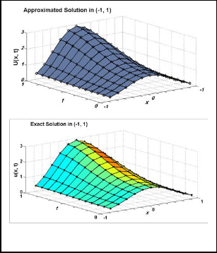
Example 3.1: Consider the linear problem (1)-(3) with the ker- nel k(x, t) = exp (-x2t) and we choose the forcing function f(x, t) so that u(x, t) = (1- x2) exp (t) is the exact solution.

 1 0 3 0

 j 

A =       



0 3 0

N −1

j 

• + = (+i ), + is a matrix with dimension
(N + 1)2 × (N + 1)(N − 1) in which the first and last (N+1)
rows are zeros, and each block matrix (𝐿𝑖 ) has a dimen- sion (N + 1) × (N + 1). The entries of (𝐿𝑖 ) can give by the
following

( i )

T(τ + 1) p

= j ( ,
− ( , )) ( ( , )) 2 ,

i +1,n

∑dk K xi τ j

k = 0

ρ τ θ

Fm ρ τ j θk

Di ,n

with (0 ≤ m ≤ M, 0 ≤ j ≤ M, 1 ≤ i ≤ N − 1, and 1 ≤ n ≤ N – 1)
respectively.
• Finally the matrix B = (Bi ), B has the dimension
(N + 1)(N − 1) × (N + 1)(N − 1). The entries of matrices (𝐵𝑖 ) is
obtained as the following

(Bi )

i ,n

T(τ j + 1) p

= ∑dk Fm (ξ(τ j ,θk ))

i ,n

4 k = 0
with (0 ≤ m ≤ M, 0 ≤ j ≤ M, 1 ≤ i ≤ N − 1, and 1 ≤ n ≤ N – 1) respectively. Each matrix in the previous equation of di- mension (N + 1) × (N + 1).
For each previous matrix we can use kronecker product to find them well.

Fig. 1. Approximated and Exact solutions respectively for x

∈ (-1, 1) and t ∈ [0, 1] at N = 12.

International Journal of Scientific & Engineering Research, Volume 5, Issue 3, March-2014 1352

ISSN 2229-5518

TABLE 1

MAXIMUM L∞ ERRORS FOR EXAMPLE (3.1)

CPU time(s) indicates the time for all calculations for the program from start to the end.

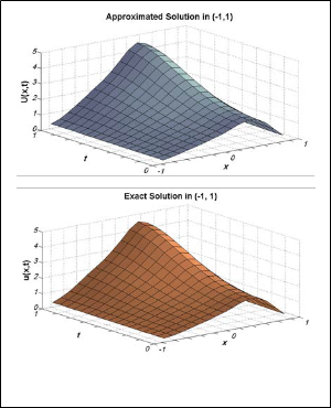
Example 3.2: Consider the linear problem (1)-(3) with the ker- nel k(x, t) = exp (-x2t) and we choose the forcing function f(x, t) so that u(x, t) = (1- x4) exp (x+t) is the exact solution.

TABLE 2

MAXIMUM L∞ ERRORS FOR EXAMPLE (3.2)

CPU time(s) indicates the time for all calculations for the program from start to the end.

Fig. 2. Approximated and Exact solutions respectively for x

∈ (-1, 1) and t ∈ [0, 1] at N = 16.

It can be seen that the errors in Tables (1)-(2) decay rapidly, which is confirmed by spectral accuracy.
All the computations are carried out in double precision arithmetic using Matlab 7.9.0 (R2009b). To obtain sufficient accurate calculations, variable arithmetic precision (vpa) is employed with digit being assigned to be 32. The code was executed on a second generation Intel Core i5-2410M, 2.3 Ghz Laptop.

4 CONCLUSION

This article used a new competitive numerical scheme based on developing Chebyshev spectral collocation method to find the approximate solution of parabolic Volterra integro- differential equations. The main advantage of using Cheby- shev scheme instead of using Legendre one is that its quadra- ture points have explicit and simple expressions as well as the corresponding weights. This enables us to avoid the complex computation of the Legendre quadrature points and the corre- sponding weights. Moreover, we made a minor modification on approximating the integration by replacing the integral function by its interpolating polynomials instead of using Gauss quadrature approximation and this increases the accu- racy of the suggested method. The numerical examples given in this work have demonstrated the potential of the newly proposed numerical scheme in solving parabolic Volterra in- tegro-differential and similar equations even with using a small number of collocation points.

REFERENCES

[1] E. G. Yanik, and G. Fairweather, “Finite element methods for parabolic and hyperbolic partial integro-differential equations”, Nonlinear Anal. (1988), 12, pp. 785–809.

[2] M. Renardy, W. Hrusa, and J. Nohel, “Mathematical Problems in Viscoelasticity”, Pitman monographs and Surveys in pure Appl. Math., New York: wiley. (1987), 35.

[3] T. A. Burton, “Volterra Integral and Differential Equations“, (second edition), Mathematics in Science and Engineering. Elsevier, vol. 202,

2005.

[4] G. Dagan, “The significance of heterogeneity of evolving scales to transport in porous formations“, Water Resour. Res., (1994), 30, pp.

3327-3337.

[5] J. Cushman, and T. Glinn, “Nonlocal dispersion in media with con- tinuously evolving scales of heterogeneity“, Transport in Porous Media, (1993), 13, pp. 123-138.

International Journal of Scientific & Engineering Research, Volume 5, Issue 3, March-2014 1353

ISSN 2229-5518

[6] R. Ewing, Y. Lin, and J. Wang, “A numerical approximation of non- Fickian flows with mixing length growth in porous media“, Acta. Math. Univ. comenian. (2001), LXX, pp. 75-84.

[7] Amiya K. Pani, and G. Fairweather, “H1-Galerkin mixed finite element methods for parabolic partial integro-differential equations”, IMA Journal of Numerical Analysis. (2002), 22, pp. 231-252.

[8] Amiya K. Pani, G. Fairweather, and Ryan I. Fernandes, “ALTERNATING DIRECTION IMPLICIT ORTHOGONAL SPLINE COLLOCATION METHODS FOR AN EVOLUTION EQUATION WITH A POSITIVE- TYPE MEMORY TERM”, SIAM J. NUMER. ANAL. (2008), 46, pp.

344-364.

[9] Amiya K. Pani, G. Fairweather, and Ryan I. Fernandes, “ADI orthogonal spline collocation methods for parabolic partial integro-differential equa- tions”, IMA Journal of Numerical Analysis. (2010), 30, pp. 248-276.

[10] F. Fakhar-Izadi, and M. Dehghan, “The spectral methods for parabol- ic Volterra integro-differential equations”, Journal of Computational and Applied Mathematics. (2011), 235, pp. 4032-4046.

[11] C. Canuto, M. Y. Hussaini, A. Quarteroni, and T. A. Zang, “Spectral Methods: Fundamentals in Single Domains”, Springer-Verlag, 2006.

[12] L. N. Trefethen, “Spectral Methods in MAT+AB”, Society for Industrial and Applied Mathematics (SIAM), Philadelphia, PA, 2000.

[13] C. Canuto, M. Y. Hussaini, A. Quarteroni, and T. A. Zang, “Spectral

Methods in Fluid Dynamics”, Springer-Verlag, 1988.

[14] W. Guo, G. Labrosse, and R. Narayanan, “The Application of the Cheby- shev-Spectral Method in Transport Phenomena”, Notes in Applied and Computational Mechanics 68, Springer-Verlag Berlin Heidelberg,

2012.

[15] J. P. Boyd, “Chebyshev and Fourier Spectral Methods”, Dover Publica- tions, Mineola, NY, 2001.

[16] J. Shen, and T. Tang, “Spectral and High-Order Methods with applica- tions”, Science Press, Beijing, China. 2006.

[17] M. Aguilar, and H. Brunner,” Collocation methods for second-order

Volterra integro-differential equations”, Appl. Numer. Math. (1988),

4, pp. 455--470.

[18] D. Conte, and B. Paternoster, “Multistep collocation methods for Volterra Integral Equations”, Applied Numerical Mathematics. (2009), 59, pp. 1721-1736.

[19] Tobin A. Driscoll, “Automatic spectral collocation for integral, in- tegro-differential, and integrally reformulated differential equa- tions”, Journal of Computational Physics. (2010), 229, pp. 5980-5998.

[20] T. Tang, “On spectral methods for Volterra integral equations and the convergence analysis”, J. Comput. Math. (2008), 26, pp. 825-837.

[21] Z. Wan, Y. Chen, and Y. Huang, “Legendre spectral Galerkin method for second-kind Volterra integral equations”, Front. Math. China. (2009), 4, pp. 181-193.

[22] Zhendong Cu, and Yanping Chen, “Chebyshev spectral-collocation method for Volterra integral equations”, Recent Advances in Scien- tific Computing and Applications, Contemporary Mathematics. (2013), 586, pp. 163-170.

[23] Wu Hua, and Zhang Jue, “Chebyshev-Collocation Spectral Method for Volterra Integro-Differential equations”, Journal of Shanghhai University (Natural Scince). (2011), 17, pp. 182-188.

[24] B. Costa, and W. S. Don, “On the computation of high order pseudo-

spectral derivatives”, Appl. Numer. Math. (2000), 33, pp. 151-159. [25] R. Baltensperger, and M. R. Trummer, “Spectral Differencing with a

twist”, J. Indus. and Appl. Math. (2003), 24, pp. 1465--1487.

[26] Elsayed M. E. Elbarbary, and Salah M. El-Sayed, “Higher order pseudospectral differentiation matrices”, Appl. Numer. Math. (2005),

55, pp. 425-438.

[27] J. S. Hesthaven, S. Gottlieb, and D. Gottlieb, “Spectral Methods for

Time-Dependent Problems”, Cambridge University Press. 21, pp. 96-

99, 2007.