International Journal of Scientific & Engineering Research, Volume 3, Issue 11, November-2012 1

ISSN 2229-5518

Assessment on Ground Control Points in Unmanned Aerial System Image Processing for Slope Mapping Studies

Khairul Nizam Tahar*1, Anuar Ahmad2, Wan Abdul Aziz Wan Mohd Akib2, Wan Mohd Naim Wan Mohd1

Abstract— The first objective of this study is to investigate the use of light weight rotary-wing UAV for mapping simulation model. The second objective is to determine the accuracy of the photogrammetric output produced from this study. In this study, the phot ogrammetric output such as stereomodel in three dimensional (3D), contour lines, digital elevation model (DEM) and orthophoto were produced from a simulation model with a dimension of 3m x 1m. In the simulation model, ground control points (GCP) and checked point (CP) were established using a total station. The GCP is used to produce photogrammetric output while the CP is used for accuracy assessment. A Nikon Coolpix consumer digital camera was used in image acquisition of the simulation model. Two methods of image capturing were used. In the first method, the camera was mounted vertically on a rotary-wing UAV and the images were captured at an altitude of 1.2 meters. In the second method, the camera was mounted vertically on a wooden structure at a fixed height (in this case 1.2 met ers). After obtaining all the required images, they were then processed using digital photogrammetric software to produce photogrammetric output. Based on the results of this study, it was found that the final product of the rotary-wing UAV was not significantly different from the results acquired from the fixed height data acquisition method. The results of this study also showed that the differences of DEM and digital orthophoto between both methods were relatively small. Finally, it can be concluded that the UAV system can be used for small-scale mapping and other diversified applications, especially for small areas, which involves a limited budget and time constraints.

Index Terms— UAV, Photogrammetry, Stereomodel, DEM, Digital Orthophoto

——————————  ——————————

1 INTRODUCTION

N 1980, a model of the rotary wing UAV was introduced to be utilized for photogrammetry work. The UAV was able to carry payloads up to 3 kg and had flying range of around 10
to 100 meters. A Rolleiflex camera unit was attached to the bottom of the UAV by installing a camera mount. A profes- sional operator was used to control for hovering operations, landing and flying the unmanned model helicopter [5]. The technology of UAV has experienced various developments over the years. According to [5], there were hundreds of UAV operated by military and civil based organizations for numer- ous applications. Demand of aerial photogrammetry has in- creased especially after the development of design, research and production of UAV platform [2], [3]. Numerous UAV's have been developed by organization or individual world- wide including a complete set of UAV which uses high quality fibers as the material for model planes [8]. UAV technology has been utilized in many applications such as farming, sur- veillance, road maintenance, recording and documentation of cultural heritage [1], [6]. Compared to other mobile systems, the UAV is the most practical solution for low budget projects with time constraints and it requires less manpower [7], [14]. Three dimensional model can be generated using UAV images after going through certain processes. The scale of aerial pho- tographs taken using UAV devices relies on flying height and focal length of digital camera as with most aerial based photo- graphs [13], [14].
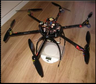
In this study, two main hardware were used which include the light weight rotary-wing UAV and high resolution digital camera. Low altitude UAV was the preferred device for data capture because it focuses on large scale mapping which in- volves small areas only. UAV's are potentially the most suita- ble equipment that can be used for this sort of project which involves very low cost budget for capturing aerial photograph of small areas. Apart from that, amateur digital camera with high resolution images was attached at the UAV. The amateur digital camera provides small sized images, which will not consume a lot of memory space. Amateur digital cameras have many different selections of resolutions which can be set on the device in which each of them will portray different pixel sizes. Figure 1 shows an example of a UAV (Hexacopter) and amateur digital camera.

(a)

————————————————

 Khairul Nizam Tahar is currently pursuing PhD in Geoinformatics in

Universiti Teknologi Malaysia, Malaysia. E-mail: nizamtahar@gmail.com

IJSER © 2012

http://www.ijser.org

International Journal of Scientific & Engineering Research, Volume 3, Issue 11, November-2012 2

ISSN 2229-5518

Fig. 1. (a) Hexacopter ; (b) Digital Camera

(b)
tioned [3], [11], [15]. The uses of Micro UAV’s have big poten- tial in forest and agricultural application as studied by Grenzdoffer et al. (2008). It is because UAV's are more flexible and able to obtain data in any weather condition [10]. The spe- cial requirement for photogrammetry and GIS (Geographical Information System) process has been studied for various ap- plications such as exterior orientation precision value, system- atic aerial survey and metric camera. There are two types of micro UAV's that has been introduced by [5] named as Carolo P330 and SUSI. Low cost micro UAV SUSI powered by 4.2kW two stroke engines, can be controlled manually by the opera- tor from the ground. The accuracy of GCP and x and y image coordinate improves when the percentage of end lap and side lap fulfill the standard block configuration. The accuracy of GCP for Z coordinate is less accurate than the GCP for X and Y
In this study, Nikon Coolpix L4 was used in acquiring simula- tion model images. Nikon Coolpix digital camera has 3x opti- cal zoom lens and a 2.0” LCD screen. In this study, Micro UAV also known as Hexacopter (Figure 1), was used in acquiring images for the stated model. Hexacopter has 6 blades in which
3 blades rotate in a clockwise direction and the other 3 blades rotate in a counterclockwise direction. The Nikon Coolpix camera was attached at the bottom of Hexacopter to capture aerial images during flight operation. The specification of the rotary wing used in this study is shown in Table 1.

TABLE 1

HEXACOPTER SPECIFICATION (RCHELI,2008)

2 RELATED WORK

Helicopter UAV has been investigated in depth for data acqui- sition as studied [4], [12]. The combination of GPS/INS and helicopter UAV increased the sensitivity of UAV to determine point of measurement on the ground as mentioned by [2], [11], [4], [13]. Many studies have been done to improve the accura- cy of GPS on board for reduction of the number of ground control needed during UAV image processing [2]. Remote control helicopters are not designed for large areas but it can be used for small areas such as areas in vicinities of complex buildings which is difficult to be captured by aircrafts of high- er speed and altitude. In addition, UAV's cost much cheaper as compared to other aircrafts or terrestrial equipment as men-
coordinates due to the systematic error in focal length with various zoom lenses [9]. The advantages of UAV are in low cost, flexible manoeuvrings, high resolution images, flying under clouds, easy launch and landing and very safe to use [15]. The disadvantages of UAV include payload limitation, small coverage for each image, increasing number of image that need to be processed and large geometric distortion.

3 METHODOLOGY

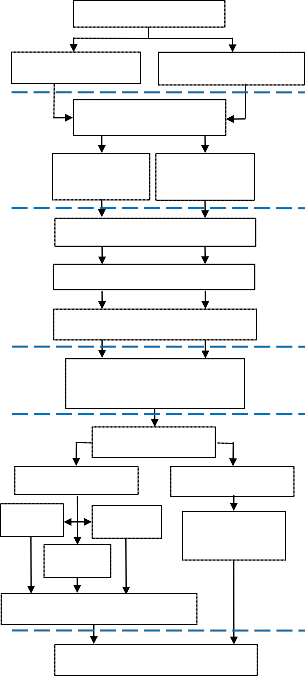
In this study, the methodology are divided into several phases namely data preparation, data collection, data processing, re- sult, analysis and discussion. Figure 2 depicts flowchart of the research methodology which concentrates on fixed platform and mobile platform. Fixed platform was built from a wooden structure that was not adjustable and it was fixed at 1.2 meter from simulated model while mobile platform using rotary wing UAV flew at altitude 1.2 meter from the simulated mod- el. Both platforms were used to obtain aerial images of simu- lated model.
The dimension of the simulated model was approximately 3 x
1 metres and was prepared using sand and cement. The simu- lated model represents a slope area along a road side which
has different gradients and slope length. The GCPs were dis- tributed on the simulated model evenly and were established using total station. Camera calibration was carried out to ob- tain all camera parameters as input for image processing. In the digital image, one of the main important values that should be considered is pixel size. Pixel size will determine the ground coverage area or size of the objects. The size of pixel involves a few elements such as number of pixel for object image, length of an object in real measurement, focal length of camera and flying height during image capturing. Further- more, each digital camera has different pixel size and it must be calculated in the flight planning phase prior to deploying the UAV. The ground coverage area of one image can be de- fined by multiplying the scale of the photograph with the resolution of the digital image. The calculation of overlap per- centage involves certain parameters such as image resolution, scale, flying height and focal length of the digital camera.

IJSER © 2012

http://www.ijser.org

International Journal of Scientific & Engineering Research, Volume 3, Issue 11, November-2012 3

ISSN 2229-5518

Simulated Model

Phase 1:

Data Preparation

tie points or three control points for each pair of overlapped photograph. The difference between fixed platform and mo- bile platform is the method of image acquisition. Fixed plat- form is built by using a stable platform while mobile platform

Flight Planning

Camera Calibration

uses a UAV to capture images. Results of the fixed platform
should be more stable and accurate as compare to the mobile
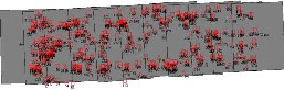
platform. The distribution of GCPs and tie points are illustrat-

Acquire Digital Images

Phase 2:

Data Collection

ed in the footprint of Figure 3 and 4 for fixed platform and mobile UAV platform respectively.

Fixed Plat- form

Mobile Plat- form

Interior Orientation Exterior Orientation Aerial Triangulation

DEM, Digital Orthophoto,

3D Model

Analysis

Phase 3:

Data Processing

Phase 4:

Result

Phase 5:

Analysis

Fig. 3. Footprint for 11 photographs of the GCPs and tie points (fixed plat- form)

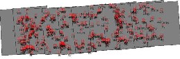
Fig. 4. Footprint for 11 photograph of the GCPs and tie points (mobile platform)

33 GCPs and 11 check points were established using a total station evenly in the simulated model. The coordinates of the GCPs were used as an accepted value or ‘true value’ for the

Image Pro- Application

purpose of accuracy assessment determination. However, 33
GCPs and 404 tie points were established during image pro-

9 GCP

19 GCP

33 GCP

Soil Loss Cal- culation

cessing for fixed platform while 33 GCPs and 353 tie points were established during image processing for mobile plat- form. Two photogrammetric results were generated after per- forming interior orientation, exterior orientation and aerial triangulation; DEM and digital orthophoto. The generated digital orthophoto for the simulated model using fixed plat-

Quantitative Assessment

Discussion & Conclusion

Fig. 2. Flowchart of the Research Methodology

Phase 6:

Conclusion

form and mobile platform are shown in Figure 5 and 6 respec- tively.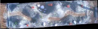

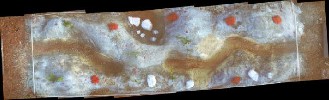
Fig. 5. Digital Orthophoto (fixed platform)

4 IMAGE PROCESSING & RESULTS

All acquired images were processed using a photogrammetric software known as Erdas Imagine software. This software re- quires camera information such as pixel size, focal length, ra- dial lens distortion and tangential distortion to carry out inte- rior orientation. All GCPs were registered during exterior ori- entation. Erdas Imagine software requires a minimum of six

Fig. 6. Digital Orthophoto (mobile platform)

IJSER © 2012

http://www.ijser.org

International Journal of Scientific & Engineering Research, Volume 3, Issue 11, November-2012 4

ISSN 2229-5518

Digital orthophotos for both platforms were compared and were found to be exactly the same except for the color which was caused by a different time exposure and temperature dur- ing image acquisition. The resulting orthophotos were the same because the residual error for both platforms was too small. The quality of DEM and digital orthophoto depends on the accuracy of GCPs. Therefore, if the quality of GCP is good, the result of DEM and digital orthophoto should also be accu- rate. The DEM for both, fixed and mobile platforms are shown in Figure 7 where the visualization of both DEMs are almost similar. In contrast, the result of DEM was found to be less accurate as compared to the orthophoto. One of the factors that affected the accuracy was the affect of motions yaw, pitch and roll during image acquisition. Configuration of GCP also plays an important role in determining the DEM result.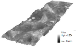


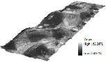
(a) (b)

Fig. 7. DEM: (a) Fixed Platform; (b) Mobile Platform

5 ANALYSIS & DISCUSSION

This study utilized a UAV system for large scale mapping. The first objective of this study is to investigate the use of light weight rotary-wing UAV for mapping a simulated model. The second objective of this study is to determine the accuracy of the photogrammetric output produced from digital image processing. It was found that the UAV system was suitable for large scale mapping with the condition that it was operated by a professional operator during data acquisition. A professional operator is needed in data acquisition in order to control the UAV during flight and to maintain the right path according to the flight planning calculation. The accuracy assessment of DEM and digital orthophotos were evaluated using root mean square error method. In the analysis section, two case studies were investigated using different number of GCP's in aerial triangulation. All acquired images from the fixed and mobile platforms were performed using two different numbers of GCP during aerial triangulation i.e. 33 GCPs, 19 GCPs and 9
GCPs. Results of fixed platform and mobile platform are illus- trated in Appendix A and Appendix B respectively. The accu- racy of the assessment of DEM and digital orthophoto was based on RMSE, mean, standard deviation and variance of sample data set after image processing. Residual errors for both platforms were also examined to analyze the accuracy of the photogrammetric products. An equation to calculate the errors in photogrammetric product is shown in equation 2.

(2)

= Estimated value
= Ground Truth value
= Error
Appendix A and B shows a sample data of checkpoint for pho- togrammetric product such as orthophoto and digital eleva- tion model. These results are illustrated more detail in Figure
8. Table 2 and 3 shows statistical results of fixed and mobile
platform respectively.

TABLE 2

STATISTICAL RESULT OF FIXED PLATFORM

AT: Aerial Triangulation; GCP: Ground Control Points; TP: Tie Points

TABLE 3

STATISTICAL RESULT OF MOBILE PLATFORM

AT: Aerial Triangulation; GCP: Ground Control Points; TP: Tie Points
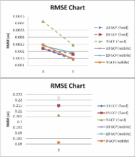
Table 2 and 3 describe the effect of different number of GCP's and tie points during image processing. These criteria are sig- nificant to determine the accuracy of the photogrammetry product using different number of GCP's and tie points during image processing. Figure 8 shows the residual mean square error chart for this study. It was found that residual errors increases with lesser number of ground control points, with an exception for the Z-axis data for mobile platform, in which the errors increase with more control points.
where,

IJSER © 2012

http://www.ijser.org

International Journal of Scientific & Engineering Research, Volume 3, Issue 11, November-2012 5

ISSN 2229-5518

(a)
Y coordinates were located along the red line 1:1. This indi- cates that the X and Y coordinates gave accurate photogram- metric results. In contrast, the Z coordinates recorded an un- derestimate and some overestimate error based on line 1:1 (red line in graph). In general, Z coordinates for 33 GCPs and
19GCPs were found to be much more precise as compared to Z coordinates with only 9 GCPs. Therefore the number of GCPs in image processing influences the accuracy and preci- sion of photogrammetric products. Apendix C and Appendix D also record minimum absolute errors (Min. AE), maximum absolute errors (Max. AE) and mean absolute errors (Mean AE). The equation of mean absolute error is as follows

Mean AE (4)

Fig. 8. RMSE Chart (a) RMSE x,y ; (b) RMSE z

(b)
where,

Mean AE = Mean Absolute Error n = Number of dataset
= Estimated value
= Measured Value
Figure 8(a) conclude that the results of RMSE for x and y co- ordinate changes when the number of control points are changed. Figure 8(b) concludes that the mean square errors between both platforms changes when the number of GCPs used in image processing is different. Number of GCPs and tie points play an important role in image processing. This result proves that the accuracy of photogrammetric product will in- crease with more GCPs. The accuracy of data can be analyzed using the linear equation as follows;
Y= a + bX (3)
Where,
Y = Measured Value
a,b = Coefficient
X = Estimated Value
Appendix C (fixed platform) and Appendix D(mobile plat- form) describe a pattern of check point error using line 1:1 (red line).Appendix C (a,b,c) shows a graph of comparison be- tween the estimated value (photogrammetric technique) and the measured value (ground truth) for X, Y and Z coordinate respectively. From Appendix C (a)(b) and (c), the error of X and Y coordinate was located along the red line which gave good accuracy while some of the Z coordinates were underes- timate and some of them were overestimate based on line 1:1 (red line in graph). It can be concluded that the Z coordinates were less accurate than X and Y coordinate. This graph also shows the effect of the number of GCPs in image processing. None of the Z coordinates were located in the red line when the GCP numbers were reduced to nine. This means that the number of GCPs contribute a significant impact in image pro- cessing for photogrammetric product.
Appendix D (a,b,c) shows a graph of comparison between the estimated value (photogrammetric technique) and the meas- ured value (ground truth) for X, Y and Z coordinate respec- tively. Based on Appendix D (a), (b) and (c), the error of X and
The result of volume determination is based on the accuracy of the slope data. Therefore, a second analysis can only be done after the accuracy of slope has been determined. The second analysis of this study involves volume determination of landslide and soil loss. The simulated model was excavated to simulate a landslide incident for large scale mapping. Fig- ure 9 shows the direction of contour lines before landslide oc- currence and after, in 3D visualization. As a result, the contour lines followed the direction of the landslide. This landslide is represented by a TIN (Triangulated Irregular Network) model for visualizing the three dimensional model of the simulated landslide. The TIN models were produced using ArcGIS 9.3 software. In general, the soil loss can be calculated by subtract- ing DEM before landslide and after landslide. Surface volume tools are available in ArcGIS 9.3 to calculate surface volume automatically. As a result the volume of soil loss was calculat- ed by subtracting the two different surface volumes before and after the landslide that was generated from both digital elevation model respectively.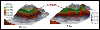

Fig.9. Superimposition between TIN and contour lines before and after landslide

The sum of soil loss of the landslide is 0.002043 meter³ and the area of landslide is 0.000026 meter². In order to prove that this result is close to the actual values, conventional method is used for comparison. The real soil loss is calculated in cylinder cube with a diameter of 23cm and 5cm in height. The volume

IJSER © 2012

http://www.ijser.org

International Journal of Scientific & Engineering Research, Volume 3, Issue 11, November-2012 6

ISSN 2229-5518

calculation in cylinder cube is 2077.38cm³ or 0.002077 meter³. The difference of volume between these two methods is
0.000034 meter³ which is about 1.64% and it is acceptable due to insignificant difference.

6 CONCLUSION

The objective of this study is to investigate the capabilities of a UAV system in slope mapping using simulated model. This study also compares the UAV data with fixed platform data to analyze the accuracy of the photogrammetric product pro- duced by both methods. It is crucial to carry out a simulated model study before conducting a real site experiment to pre- dict the outcome. In this study, it was found that the light weight rotary-wing UAV was successfully used for capturing the images of the simulated model for small-scale mapping. The digital images were successfully processed to generate DEM. Future study could be carried out using various flying heights and subsequently determine the accuracy. This study also shows that the accuracy of the photogrammetric output from both types of platforms are similar. It is anticipated that the results could change if different flying is used for both platform since this study covers almost the same flying heights and the distance from the simulated model for both the mobile and the fixed platform, in which they were both at low heights and close to the object. Finally, it can be concluded that the UAV could be used for small-scale mapping as demonstrated in this study

ACKNOWLEDGMENT

Faculty of Architecture, Planning and Surveying Universiti Teknologi MARA (UiTM) and Faculty of Geoinformation & Real Estate, Universiti Teknologi Malaysia (UTM) are greatly acknowledged.

REFERENCES

[1] M. Bryson and S. Sukkarieh, “Architecture for Cooperative Airborne Simu- lataneous Localization and Mapping,” Journal of Intelligent Robot System, vol. 55, pp. 267-297, 2009.

[2] A. Cesetti, E. Frontoni, A. Mancini, A. Ascani, P. Zingaretti, and S. Longhi, “A Visual Global Positioning System for Unmanned Aerial Vehicles Used In Photogrammetric Applications,” Journal of Intelligent Robot System, vol. 61, pp. 157-168, 2011.

[3] H.Y. Chao, Y.C. Cao, and Y.Q. Chen, “Autopilots for Small Unmanned Aerial

Vehicles: A Survey,” International Journal of Control, Automation and Sys- tems, vol. 8, no. 1, pp. 36-44, 2010.

[4] U. Coppa, A. Guarnieri, F. Pirotti, and A. Vettore, “Accuracy Enhancement Of

Unmanned Helicopter Positioning With Low-Cost System,” Applied Geo- matic, vol. 1, pp. 85-95, 2009.

[5] G.J. Grenzdoffer, A. Engel, and B. Teichert, “The Photogrammetric Potential of Low Cost UAVs in Forest and Agriculture,” The International Archives of the Photogrammetry, Remote Sensing and Spatial Information Sciences, Vol. XXXVII. Part B1. Beijing, China, 2008.

[6] A. Hervouet, R. Dunford, H. Piegay, B. Belletti, and M.L. Tremelo, “Analysis of Post-Flood Recruitment Patterns In Braided-Channel Rivers At Multiple Scales Based On An Image Series Collected By Unmanned Aerial Vehicles, Ultra-Light Aerial Vehicles And Satellites,” Geographical Information Science

& Remote Sensing, vol. 48, no. 1, pp. 50-73, 2011.

[7] A. Jaakkola, J. Hyyppa, A. Kukko, X. Yu, H. Kaartinen, M. Lehtomaki, and Y.

Lin, “A Low-Cost Multi-Sensoral Mobile Mapping System And Its Feasibility For Tree Measurements,” International Society for Photogrammetry and Re- mote Sensing Journal of Photogrammetry and Remote Sensing, vol. 65, pp.

514-522, 2010.

[8] B. Li, X. Sheng, A. Xia, E. Chengwen, and B. Li, “Actualize of Low Altitude Large Scale Aerophotography and Geodesic base on Fixed-wing Unamanned Aerial Vehicle Platform,” The International Archives of the Photogrammetry, Remote Sensing and Spatial Information Sciences, Vol. XXXVII. Part B1. Bei- jing, China, 2008.

[9] F. Remondiono, and C. Fraser, “Digital Camera Calibration Methods: Con-

siderations and Comparisons,” International Society for Photogrammetry and Remote Sensing Commission V Symposium Image Engineering and Vision Metrology. International Archives of Photogrammetry and Remote Sensing, vol. XXXVI, Part 5, pp. 266-272, 2006.

[10] D.G. Schmale III, B.R. Dingus, and C. Reinholtz, “Development and Applica- tion of An Autonomous Unmanned Aerial Vehicle For Precise Aerobiological Sampling Above Agricultural Fields,” Journal of Field Robotics, vol. 25, no. 3, pp. 133-147, 2008.

[11] K. Schwarz, and N. El-Sheimy, “Mobile Mapping System- State of the Art and the Future Trends Istanbul,” International Archives of Photogrammetry and Remote Sensing, vol. XXXV, Part B1, 2004.

[12] D.H. Shim, J.S. Han, and H.T. Yeo, “A Development of Unmanned Helicop-

ters for Industrial Applications,” Journal of Intelligent Robot System, vol. 54, pp. 407-421, 2009.

[13] K.N. Tahar and A. Ahmad, “Capability of Low Cost Digital Camera for Pro- duction of Orthophoto and Volume Determination,” 7th International Collo- quium on Signal Processing & Its Applications IEEE, Penang, Malaysia, 2011.

[14] K.N. Tahar, A. Ahmad and W.A.A. Wan Mohd Akib, “Unmanned Aerial Vehicle Technology for Low Cost Landslide Mapping,” 11th South East Asian Survey Congress and 13thInternational Surveyor’s Congress, Putra World Trade Centre, Kuala Lumpur, Malaysia, 2011.

[15] L. Yan, Z. Gou, and Y. Duan, “A UAV Remote Sensing System: Design and Tests: Geospatial Technology for Earth Observation Data”, (eds) Li Deren, Shan Jie, Gong Jianya. New York : Springer-Verlag, 2011.

IJSER © 2012

http://www.ijser.org

International Journal of Scientific & Engineering Research, Volume 3, Issue 11, November-2012 7

ISSN 2229-5518

Appendix A : Residual Error (Fixed Platform)

33 Ground Control Point

19 Ground Control Point

9 Ground Control Point

IJSER © 2012

http://www.ijser.org

International Journal of Scientific & Engineering Research, Volume 3, Issue 11, November-2012 8

ISSN 2229-5518

Appendix B: Residual Error (Mobile Platform)

33 Ground Control Point

19 Ground Control Point

9 Ground Control Point

IJSER © 2012

http://www.ijser.org

International Journal of Scientific & Engineering Research, Volume 3, Issue 11, November-2012 9

ISSN 2229-5518

Appendix C: Fixed Platform (a) 33 GCPs ; (b) 19 GCPs ; (c) 9 GCPs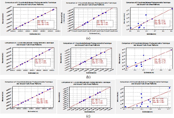

IJSER © 2012

http://www.ijser.org

International Journal of Scientific & Engineering Research, Volume 3, Issue 11, November-2012 10

ISSN 2229-5518

Appendix D: Mobile Platform (a) 33 GCPs ; (b) 19 GCPs ; (c) 9 GCPs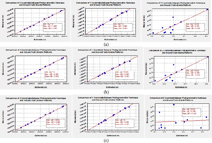

IJSER © 2012

http://www.ijser.org