Stanford University in 1950‘s.

Inte rnatio nal Jo urnal o f Sc ie ntific & Eng inee ring Re se arc h, Vo lume 3, Issue 2, February -2012 1
ISS N 2229-5518
Mr.Paduri Veerabhadram , Mrs.Antoinette Lombard, Dr Pieter Conradie
Departm ent Of Infor mation Com munication T echnolog y
Vaal Uni versity Of Techn olog y
Vand erb ejilpark, Private Ba g
Email: pa duri72@sa ym ail.co.za, vp aduri@g mail.com
—————————— ——————————
The original inspiration for the term ―Artificial Neural
Network ― came from examination of central nervous systems and their neurons, axons, dendrites, and synapses, which constitute the processing elements of biological neural networks investigated by neuroscience. In an artificial neural network, simple artificial nodes, variously called "neurons", "neurodes", "processing elements" (PEs) or "units", are connected together to form a network of nodes mimicking the biological neural networks hence the term "artificial neural network".
Because neuroscience is still full of unanswered questions, and since there are many levels of abstraction and therefore many ways to take inspiration from the brain, there is no single formal definition of what an artificial neural network is. Generally, it involves a network of simple processing elements that exhibit complex global behavior determined by connections between processing elements and element parameters. While an artificial neural network does not have to be adaptive per se, its practical use comes with algorithms designed to alter the strength (weights) of the connections in the network to produce a desired signal flow.These networks are also similar to the biological
Many task which seem simple for us, such as reading a
handwritten note or recognizing a face, are difficult task for even the most advanced computer. In an effort to increase the computer ability to perform such task, programmers began designing software to act more like the human brain, with its neurons and synaptic connections. Thus the field of
―Artificial neural network‖ was born. Rather than employ the traditional method of one central processor (a Pentium) to carry out many instructions one at a time, the Artificial neural network software analyzes data by passing it
neural networks in the sense that functions are performed collectively and in parallel by the units, rather than there being a clear delineation of subtasks to which various units are assigned (see also connectionism). Currently, the term Artificial Neural Network (ANN) tends to refer mostly to neural network models employed in statistics, cognitive psychology and artificial intelligence. Neural network models designed with emulation of the central nervous system (CNS) in mind are a subject of theoretical neuroscience and computational neuroscience.
In modern software implementations of artificial neural networks, the approach inspired by biology has been largely abandoned for a more practical approach based on statistics and signal processing. In some of these systems, neural networks or parts of neural networks (such as artificial neurons) are used as components in larger systems that combine both adaptive and non -adaptive elements. While the more general approach of such adaptive systems is more suitable for real-world problem solving, it has far less to do with the traditional artificial intelligence connectionist models. What they do have in common, however, is the principle of non -linear, distributed, parallel and local processing and adaptation.
through several simulated processos which are
interconnected with synaptic like ―weight‖
Once we have collected several record of the data we wish to analyze, the network will run through them and ―learn ‖ the input of each record may be related to the result. After training on a few doesn‘t cases the network begin to organize and refines its on own architecture to feed the data to much the human brain; learn from example.
IJSER © 2012 http :// www.ijser.org
Inte rnatio nal Jo urnal o f Sc ie ntific & Eng inee ring Re se arc h, Vo lume 3, Issue 2, February -2012 2
ISS N 2229-5518
network was pioneered by BERNARD WIDROW of
Stanford University in 1950‘s.
Why would anyone want a `new' sort of computer?
What are (everyday) computer systems good at... .....and not so good at?
Fast arithmetic Interacting with noisy data or data from the environment
Doing precisely what the programmer programs them to do Massive parallelism Massive parallelism Fault tolerance
Adapting to circumstances
Where can neural network systems help?
where we can't formulate an algorithmic solution.
where we can get lots of examples of the behaviour we require.
where we need to pick out the structure from existing data.
What is a neural network?
Neural Networks are a different paradigm for computing:
Von Neumann machines are based on the processing/memory abstraction of human information processing.
Neural networks are based on the parallel architecture of animal brains.
Neural networks are a form of multiprocessor computer system, with
Simple processing elements
A high degree of interconnection
Simple scalar messages
Adaptive interaction between elements
A neural network acquires knowledge through learning.A neural network‘s knowledge is stored with in the interconnection strengths known as synaptic weight.
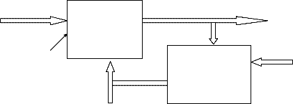
Neural network are typically organized in layers . Layers
are made up of a number of interconnected ‗nodes‘, which contain an ‗activation function‘. Patterns are presented to the network via the ‗input layer‘, which communicates to one or more ‗hidden layers‘ where the actual processing is done via a system of weighted ‗connections‘. The hidden layers then link to an ‗output layer‘ where the answer is output as shown in the graphic below.
Hidden Layers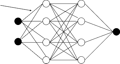
Connections
Input layer Output layer
Basic structure of neural network
IJSER © 2012 http :// www.ijser.org
Inte rnatio nal Jo urnal o f Sc ie ntific & Eng inee ring Re se arc h, Vo lume 3, Issue 2, February -2012 2
ISS N 2229-5518
Each layer of neural makes independent computation on data that it receives and passes the result to the next layers(s). The next layer may in turn make independent computation and pass data further or it may end the computation and give the output of the overall computation .The first layer is the input layer and the last one, the output layer. The layers that are placed within these two are the middle or hidden layers.
A neural network is a system that emulates the cognitive abilities of the brain by establishing recognition of particular inputs and producing the appropriate output. Neural networks are not ―hard-wired‖ in particular way; they are trained using presented inputs to establish their own internal weights and relationships guided by feedback. Neural networks are free to form their own internal working and adapt on their own. Commonly neural network are adjusted, or trained so that a particular input leads to a specific target output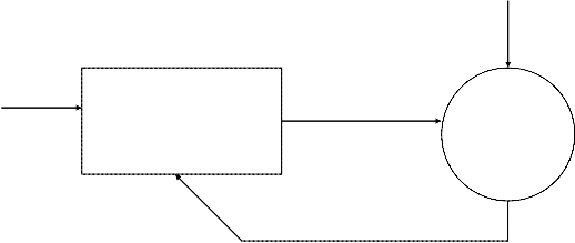
Target
Input
Neural network Includ ing connections (called weights)
Compare
Figure showing adjust of neural network
There, the network is adjusted based on a comparison of the output and the target, until the network output matches the target. Typically many such input/target pairs are used to train network.
Once a neural network is ‗trained‘ to a satisfactory level it may be used as an analytical tool on other data. To do this, the user no longer specifies any training runs and instead allows the network to work in forward propagation mode only. New inputs are presented to the input pattern where they filter into and are processed by the middle layers as
though training were taking place, however, at this point the output is retained and no back propagation occurs.
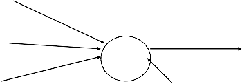
Nervous system of a human brain consists of neurons,
which are interconnected to each other in a rather complex way. Each neuron can be thought of as a node and interconnection between them are edge, which has a weight associates with it, which represents how mach the tow neuron which are connected by it can it interact.
Node (neuron)
Edge interconnection
IJSER © 2012 http :// www.ijser.org
Inte rnatio nal Jo urnal o f Sc ie ntific & Eng inee ring Re se arc h, Vo lume 3, Issue 2, February -2012 2
ISS N 2229-5518
Functioning of A Nervous System
The natures of interconnections between 2 neurons can
such that – one neuron can either stimulate or inhibit the other. An interaction can take place only if there is an edge between 2 neurons. If neuron A is connected to neuron B as below with a weight w, then if A is stimulated sufficiently, it sends a signal to B. The signal depends on![]()
W A B
The weight w, and the nature of the signal, whether it is stimulating or inhibiting. This depends on whether w is positive or negative. If its stimulation is more than its threshold. Also if it sends a signal, it will send it to all nodes to which it is connected. The threshold for different neurons may be different. If many neurons send signal to A, the combined stimulus may be more than the threshold. Next if B is stimulated sufficiently, it may trigger a signal to all neurons to which it is connected.
Depending on the complexity of the structure, th e overall functioning may be very complex but the functioning of individual neurons is as simple as this. Because of this we may dare to try to simulate this using software or even special purpose hardware.
Major components Of Artificial Neuron
This section describes the seven major components, which
make up an artificial neuron. These components are valid whether the neuron is used for input, output, or is in one of the hidden layers.
A neuron usually receives many simultan eous inputs. Each
input has its own relative weight, which gives the input the impact that it needs on the processing elements summation function. These weights perform the same type of function, as do the varying synaptic strengths of biological neurons. In bath cases, some input are made more important than others so that they have a greater effect on the processing element as they combine to produce a neuron response. Weights are adaptive coefficients within the network that determine the intensity of the input signal as registered by the artificial neuron. They are a measure of an input‘s connection strength. These strengths can be modified in response to various training sets and according to a network‘s specific topology or through its learning rules. Component 2. Summation Function:
The first step in a processing element‘s operation is to
compute the weighted sum of all of the inputs. Mathematically, the inputs and the corresponding weights are vectors which can be represented as
{ i1, i2,i3,………….in } and {w1, w2,w3,……………….wn}. The total input signal is the dot, or inner, product of these two vectors. This simplistic summation function is found by multiplying each component of the i vector by the corresponding component of the w vector and then adding up all the products.
Input1 = i1*w1,
input2=i2*w2, etc., are added as
{input1+input2+input3………..+ input n } .
The result is a single number, not a multi-element vector.
Geometrically, the inner product of two vectors can be considered a measure of their similarity. If the vector point in the same direction, the inner product is maximum; if the vectors points in opposite direction (180 degrees out of phase), their inner product is minimum. The summation function can be more complex than just the si mple input and weight sum of products. The input and weighting coefficients can be combined in many different ways before passing on to the transfer function. In addition to a simple product summing, the summation function can select the minimum, maximum, majority, product, or several normalizing algorithms. The specific algorithm for combining neural inputs is determined by the chosen network architecture and paradigm.
The result of the summation function, almost always the weighted sum, is transformed to a working out put through an algorithm process known as the transfer function. In transfer function the summation total can be compared with some threshold to determine the neural output. If the sum is greater than the threshold value, the processing element generates a signal. If the sum of the input and weight product is less than the threshold, no signal (no some inhibitory signal) is generated. Both types of response are significant.
A simple binary neuron with 3 inputs ( X [1], X [2] and X [3]) and 2 outputs (O [1] and O[2] ). Every neuron has a particular threshold. A neuron fires only if the weighted sum of its input exceeds the threshold.
Sum=summation {W i * Xi } If sum>=T then the output is
Output O[1] and O[2]= 1 if { X[i] * W[i] >=T } = 0 else
IJSER © 2012 http :// www.ijser.org
Inte rnatio nal Jo urnal o f Sc ie ntific & Eng inee ring Re se arc h, Vo lume 3, Issue 2, February -2012 1
ISS N 2229-5518
X [1] W [1]
X [2] W [2] (synaptic connection)
O [1]
X [3] W [3]
(neuron processing node)
McCulloch-Pitts Neuron Model
We can use different kind of threshold functions namely: Sigmoid function : f (x)=1/(1+exp(-x))
Step function : f (x) =0 if x<T
=k if x>=T Ramp funtion : f (x)=ax+b
The transfer function could be something as simple as depending upon whether the result of the summati on function is positive or negative. The network could output zero and one, and minus one, or other numeric combinations. The transfer function would then be a ―hard limiter‖ or step function.
Hard limiter Ramping function
Y y 1
1 x x
-1 -1 x<0, y=-1 x<0, y=0 x>=0, y=1 0<=x<=1, y=x
x>1, y=1
y sigmoid functions y
1 1
x x
-1,0
y = 1/(1+e-x) x>=0, y=1-1(1+x)
x<0, y=-1+1(1-x)
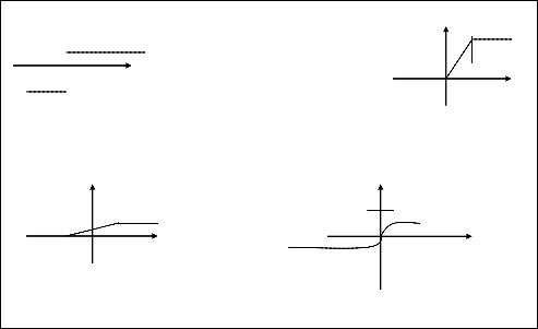
Figure : Sample Transfer Functions
directly equivalent to the transfer function‘s result. Some
After the processing element‘s transfer function, the result can pass through additional processes which scale and limit. This scaling simply multiplies a scale factor times the transfer value, and then adds an offset. Limiting is the mechanism, which ensures that the scaled result does not exceed, and upper or lower bound. This limiting is in addition to the hard limits that the original transfer function may have performed.
At Each processing element is allowed one output signal,
which it may output to hundreds of other neurons. This is the just like the biological neuron, where there are many inputs and only one output action. Normally, the output is
network topologies, however, modify the transfer result to incorporate competition among neighboring processing elements. Neurons are allowed to complete with each other, inhibiting processing elements unless they have great strength. Competition can occur one or both of two levels. First, competition determines which artificial neuron will be active, are provides an output. Second, competitive inputs help determine which processing elements will participate in the learning or adaptation process. Component 6: Error function and back-propagated value: In most learning networks the difference between the current output and the desired output is calculated. This raw error is then transformed by the error function to
IJSER © 2012 http :// www.ijser.org
Inte rnatio nal Jo urnal o f Sc ie ntific & Eng inee ring Re se arc h, Vo lume 3, Issue 2, February -2012 2
ISS N 2229-5518
match particular network architecture. The most basic architectures use this error directly, but some square the error while retaining its sign, some cube the error, other paradigms modify the raw error to fit their specific purposes. The artificial neuron‘s error is then typically propagated into the learning function of another processing element. This error term is sometimes called the current error.
The current error is typically propagated backwards to a previous layer. Yet, this back-propagated value can be either the current error, the current error scaled in some manner (obtained by the derivative of the transfer function), or some desired output depending on the network type. Normally, this back-propagated value, after being scaled by the learning function, is multiplied against each of the incoming connection weights to modify them before the next learning cycle.
The purpose of the learning function is to modify the
variable connection weights on the inputs of each processing elements according to some neural base algorithm. This process of changing the weights of the inputs connections to achieve some desired results could
also be called the adaption function, as well as the lea rning mode.
Paradigms of learning
There are three broad paradigms of learning:
Supervised
Unsupervised (or self-organised)
Reinforcement learning ( a special case of supervised learning ).
The vast majority of the artificial neural network solutions have been trained with supervision. In this mode, the actual output of a neural network is compared to the desired output. The network then adjusts weights, which are usually randomly set to begin with, so that the next iteration, or cycle, will produce a closer match between the desired and the actual output. This learning method tries to minimize the current errors of all processing elements. This global error reduction is created over time by continuously modifying the input weights until acceptable network accuracy is reached.
Adaptive
W
![]()
Distant generator
Learning signal
D
Ρ [d, 0] Distance measure
Block dig. Of supervised learning
In supervised learning the system directly compares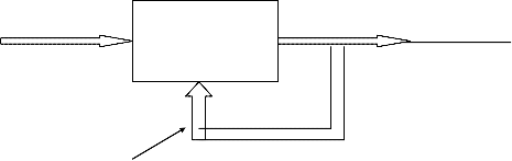
the network output with a known correct or desired answer, whereas in unsupervised learning the output is not known. Unsupervised training allows the neurons to compete with each other until winner emerge. The resulting values of the winner neurons determine the class to which a particular data set belongs.
Adaptive
X network
O
W
Unsupervised learning is the great promise of the future. It shouts that computers could some day learn on their own in a true robotic sense. Currently, this learning method is limited to networks known as self organizing map. These kinds of networks are not in wide spread use.
Block diagram of unsupervised learning
Reinforcement learning is a form of supervised learning where adopted neuron receives feedback from the environment that directly influences learning.
IJSER © 2012 http :// www.ijser.org
Inte rnatio nal Jo urnal o f Sc ie ntific & Eng inee ring Re se arc h, Vo lume 3, Issue 2, February -2012 2
ISS N 2229-5518
Learning law :
The following general learning rules is adopted in the
neural network studies: The weight vector
wi ={Wi1, Wi2…………………Win}t increases proportion to the product of input x and learning signal r.
of the teacher‘s signal di.
Hence we have, r =r (Wi, X, di) and increment in weight vector produced by the learning step at time t is Wi (t)
=cr [Wi (t), X (t), di (t)] X (t)
Where c is learning constant.
Thus Wi (t+1) =Wi (t)+ cr [Wi (t), X (t), di (t)] X (t) Various learning rules are their assist the learning process.
They are :
1.Hebbian learning rule :
This rule represents purely feed forward,
unsupervised learning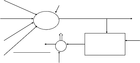
X1 Wi1 ith neuron
X2 Wi2 Oi
Wi3 ΔWi
X3 di
Win x
r
Xn
c
Hebbian Learning Rule
Learning signal generate
According to this rule, we have r=f(Wti, X)
and increment of weight becomes
Wi=c f(Wti, X) X
In this learning, the initial weight of neuron is.
This learning is supervised and learning signal is equal to
r =di-Oi
Where Oi=sgn(Wti, X) and di is the desired response. Weight adjustment in this method is
Wi=c[di- sgn(Wti, X)] X
in this method of learning, initial weight can have any value and neuron much be binary bipolar are binary unipolar.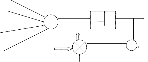
X1
X2 Wi1 TLU Wi2 neti
oi
Wi3
+ΔWi
X3
Win di-oi di
Xn X +
C
Perception Learning Rule
IJSER © 2012 http :// www.ijser.org
Inte rnatio nal Jo urnal o f Sc ie ntific & Eng inee ring Re se arc h, Vo lume 3, Issue 2, February -2012 2
ISS N 2229-5518
This rule is valid for continuous activation functions and in the supervised training mode. The learning signal is called as delta and is given as:
r=[di – f(Wti X)] f (Wti X)
The adjustment for the single weight in this rule is given as:
Wi = c (di-Oi) f (net i) X
In this method of learning, the initial weight can have any value and the neuron must be continuous.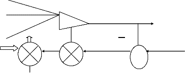
X1
Wi1 continuous perception
X2 Wi2 (neti) Oi
Win
Xn ΔWi f΄(net i)
+
X
c
Delta Learning Rule
r di - oi + di
This is applicable for the supervised training of neural
networks and is independent of activation function. Learning signal is given as :
r = di – Wti X
The weight vector increment under this learning rule is
:
Wi=c (di - Wti X) X
Substituting r = di in general learning rule, we obtain correlation learning rule. The adjustment for the weight vector is given by:
Wi = c di X
This rule is applicable for an ensemble of neurons, let‘s
say being arranged in a layer of p units. This learning is base on the premise that one of the neurons in the layer, say the mth, has the maximum response due to input x, as shown in fig. This neuron is declared the winner. As a result of this winning event, the weight vector Wm containing weights
W11
X1 Wm1 O1
Wp1 ―winning neuron‖
W1j
Xj Wmj Om
Wpj
W1n Wmn
Xn Wpn Op
Winner –take –All learning Rule
highlight in the fig. , by double headed arrow, is the only one adjusted in the given unsupervised learning. It‘s increment is computed as follows:
This is an another learning rule that is best explained when the neurons are arranged in layers. This rule is designed to produce a desired response d of the layer of p neurons as shown in fig… This rule is concern ed with the supervised learning and the weight adjustment is computed as:
IJSER © 2012 http :// www.ijser.org
Inte rnatio nal Jo urnal o f Sc ie ntific & Eng inee ring Re se arc h, Vo lume 3, Issue 2, February -2012 2
ISS N 2229-5518
X W11 o1
Wm1
Wp1 ΔWi +
W1j β
+ d1
Xj Wmj om
Wpj
+ dm
W1n Wmn β
Xn op
Wpn ΔWi +
β +
Outstar Learning Rule
Training a neural network:
Since the output of the neural network may not be what is expected, the network needs to be trained. Training involves altering the interconnection weights between the neurons. A criterion is needed to specify when to change the weights and how to change them. Training is an external process whiling learning is the process that takes place internal to the network. The following guideline will be of help as a step methodology for training a network.
Choosing the number of neurons
The number of hidden neurons affect how well the network is able to separate the data. A large number of hidden neurons will ensure correct learning and the network is able to correctly predict the data it has been trained on, but its performance on new data, its ability to generalize, is compromised. With too few hidden neurons, the network may be unable to learn the relationship amongst the data and the error will fail to fall below an acceptable level. Thus, selection of the number of hidden neurons is a crucial decision. Often a trial and error approach is taken starting with a modest number of hidden neurons and gradually increasing the number if the network fails to reduce its error. A much used approximation for the number of hidden neurons for a three layered network is N=1/2(j + k)+v P, where J and K are the number of input neurons and P is the number of patterns in the training set.
Choosing the initial weights
The learning algorithm uses steepest descent technique,
which rolls straight downhill in weight space until the first valley is reached. This valley may not correspond to a zero error for the resulting network. This makes the choice of initial starting point in the multidimensional weight space critical. However, there are no recommended rules for th is selection except
trying several different weight values to see if the network results are improved.
Choosing the learning rate
Learning rate effectively controls the size of the step that is taken in multidimensional weight space when
each weight is modified. If the selected learning rate is too large then the local minimum may be over stopped constantly, resulting in oscillations and slow convergence to lower error state. If the learning rate is too low, the number of iterations requires may be too large, resulting in slow performance. Usually the default value of most commercial neural network packages are in the range 0.1 -
0.3 providing a satisfactory balance between the two
reducing the learning rate may help improve convergence to a local minimum of the error surface.
Choosing the activation function
The learning signal is a function of the error multiplied by the gradient of the activation
function df/d (net). The larger the value of the gradient, the more weight the learning will receive. For training, the activation function must be monotonically increasing from left to right, differentiable and smooth.
Models Of artificial Neural Networks
There are different kinds of neural network models
that can be used. Some of the common ones are:
This is a very simple model and consists of a single ‗trainable‘ neuron. Trainable means that its threshold and input each input has a desired output (determined by us). If the neuron doesn‘t gives the desired output, then it has made a mistake. To rectify this, its threshold and/or input weights must be changed. How this change is to be calculated is determined by the learning algorithm.
IJSER © 2012 http :// www.ijser.org
Inte rnatio nal Jo urnal o f Sc ie ntific & Eng inee ring Re se arc h, Vo lume 3, Issue 2, February -2012 2
ISS N 2229-5518
The output of the perceptron is constrained to Boolean values – (true, false), (1, 0), (1, -1) or whatever. This is not a limitation because if the output of the perceptron were to be the input for something else,
then the output edge could be made to have a weight. Then the output would be dependant on this weight. The perceptron looks like –
X1 W1
1
X2 W2
X3 W3
y
Xn Wn
X1, X2, …………., Xn are inputs. These could be real numbers or Boolean values depending on the problem. y is the output and is Boolean.
w 1, w2, …………, wn are weights of the edges and are real valued.
T is the threshold and is a real valued.
The output y is 1 if the net input which is :
w1 x1 + w2 x2 + …….+ wn xn
is greater than the threshold T. Otherwise the output is zero.
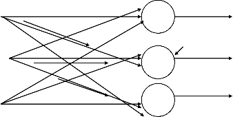
Elementary feed forward architecture of m
neurons and receiving n inputs is shown in the figure. Its output and input vectors are respectfully.
O = [O] O2 ………Om]
X = [x] x2………..xn]
Weight Wij connects the ith neuron with the jth input.
Hence activation value net i for the ith neuron is
W11
Net i = j=1n Wij Xj
for i=1, 2, 3,……, n
Hence, the output is given as
Oi = f(Wti X) for i = 1,
2, 3, ……….., m
Where Wi is the weight vector containing the weights leading towards
the ith output node and defined as
Wi = [Wi1 Wi2 …………. Win]
If is the nonlinear matrix operarte, the mapping of input space X to output space O implemented by the network can be expressed
O = WX
Where W is the weight matrix, also called the
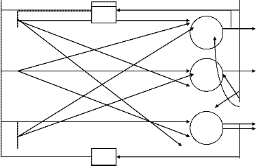
connection matrix.The generic feed forward network is characterized by the lack of feedback. This type network can be connected in cascade to create a multiplayer network.
X1 W21 O1
W12 1
X2 W22
W2n O2
Wm1 2
W1n Wm2
Xn Wmn m On
X(t)
┌ [Wx]
O(t)
Single –layer Feed forward network: interconnection scheme & block dig.
![]()
W11 W12 ……..……W1n
IJSER © 2012 http:// www.ijser.org
Inte rnatio nal Jo urnal o f Sc ie ntific & Eng inee ring Re se arc h, Vo lume 3, Issue 2, February -2012 2
ISS N 2229-5518
W21 W22 ……..……W2n
…………… ……………
W = ………………………….
Wm1 ……………….Wmn![]()
┌ [.] =![]()
![]()
![]()
f(.) O…………….O
O f (.) ………..O
. . ………… .
. . ………… .
O O………….f(.)
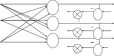
A feedback network can be obtained from the feedforawrd network by connecting the neuron‘s outputs to their inputs, as shown in the fig. The essence of closing the feedback loop is to hold control of output Oi through outputs Oj; for j =1, 2, ……, m. or
O(t+ Δ) = ┌[W o(t)]
controlling the output at instant t+Δ by the output at instant t. This delay Δ is introduced by the dela y element in the feedback loop. The mapping of O(t) into O(t+ Δ) can now be written as
O2 (t)
W11
O1 (t)
X1 W21 O1(t+ Δ)
W12
x2 W22 O2(t+ Δ) W2n
W1n Wm1
Wm2
Lag free neuron
Xn Wmn O3(t+ Δ)
m
Om(t) Δ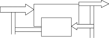
X (0) O (t+∆)
Instantaneous
O (t)
network
Delay
Single –layer feedback network : interconnection scheme & block dig.
Notations Used:
M1 is a 2-D matrix where M1[i] [j] represents the weight on the connection from the ith input neuron to the jth neuron in
the hidden layer.
M2 is a 2 –D matrix where M2[i][j] denotes the weight on the connection from the ith hidden layer neuron to the jth output layer neuron.
x, y and z are used to denote the outputs of neurons from the input layer, hidden layer and output layer respectively.
If there are m input data, then (x1, x2, ……., xm). P denotes the desired output pattern with components (p1, p2, ………, pr) for r outputs.
IJSER © 2012 http :// www.ijser.org
Inte rnatio nal Jo urnal o f Sc ie ntific & Eng inee ring Re se arc h, Vo lume 3, Issue 2, February -2012 2
ISS N 2229-5518
Let the number of hidden layer neurons be n. βo = learning parameter for the output layer. βh = learning parameter for the hidden layer. α = momentum term
θj = threshold value (bias) for the jth hidden layer neuron.
τj = threshold value for the jth output layer neuron. ej = error at the jth output layer neuron.
tj = error at the jth hidden layer neuron.
Threshold function = sigmoid function : F(x) = 1/(1 +
exp(x)).
Output of jth hidden layer neuron : yj = f((Σi xi
M1[i][j]) + θj)
Output of jth output layer neuron : zj = f((Σi yi M2[i][j]) + τj). ith component of vector of output differences:
desired value – computed value = Pj – zj
ith component of output error at the output layer:
ej = pj – zj.
ith component of output error at the hidden layer:
ti = yi (1 – yi ) (Σj M2[i][j ] ej )
Adjustment of weights between the ith neuron in the hidden layer and jth output neuron:
ΔM2[i][j] (t) = β0 yi ej + α ΔM2 [i][j ] (t -1)
Adjustment of weights between the ith input neuron and jth
neuron in the hidden layer :
ΔM1[i][j] = βh xi tj + α ΔM1 [i][j] (t - 1) Adjustment of the threshold value for the jth output neuron:
Δ τj = β0 ej
Adjustment of the threshold value for the jth hidden layer
neuron:
Δ θj = βh ej
Neural network applications:
High performance aircraft autopilot, flight
path simulation, aircraft control systems, autopilot enhancements, aircraft component simulation, aircraft component fault detection.
Automobile automatic guidance system, warranty activity analysis.
Check and other document reading credit
application evaluation.
Neural networks are used to spot unusual credit card activity that might possibly be associated with loss of a credit card
Weapon steering, target tracking, object discrimination, facial recognition, new kinds of sensors, sonar, radar and image signal
processing including data compression, feature extraction and noise suppression, signal/ image identification.
Code sequence prediction, integrated circuit chip laying, process control, chip failure analysis, machine vision voice synthesis,
nonlinear modeling.
Animation, special effects, market forecasting.
Real estate appraisals, loan advisor, mortgage
screening, corporate bond rating, credit-line use analysis, and portfolio trading program, corporate financial analysis, and currency price prediction.
Neural networks are being trained to predict the output gasses of furnaces and other industrial process. They then replace complex
and costly equipment used for this purpose in the past.
Neural networks are used in policy application evaluation, product optimization.
Neural networks are used in manufacturing process control, product design and analysis, process and machine diagnosis, real-time particle identification, visual quality analysis, paper quality prediction, computer – chip quality analysis, analysis of grinding operations, chemical product design analysis,
machine maintenance analysis, project bidding, planning and management, dynamic modeling of chemical process system.
Neural networks are used in breast cancer cell analysis, EEG and ECG analysis, prosthesis design, optimization of transplant times, hospital expense reduction, hospital quality
improvement, and emergency room test advisement.
Neural networks are used in exploration of oil
and gas.
Neural networks are used in trajectory control, forklift robot, manipulator controllers, vision systems
Artificial intelligence
Character recognition
Image understanding
Logistics
Optimization
Quality Control
Visualization
IJSER © 2012 http :// www.ijser.org
Inte rnatio nal Jo urnal o f Sc ie ntific & Eng inee ring Re se arc h, Vo lume 3, Issue 2, February -2012 3
ISS N 2229-5518
Advantages and disadvantages Of ANN:
It involve human like thinking.
They handle noisy or missing data.
They create their own relationship amongst
information – no equations!
They can work with large number of variables
or parameters.
They provide general solutions with good
predictive accuracy.
System has got property of continuous
learning.
They deal with the non-linearity in the world
in which we live.
In learning process time required may be in several months or years.
It is hard to implement
Artificial neural network, in the present scenario is novel in
it‘s technological field and still we have to witness a large of it‘s development in the upcoming era‘s, whose speculations are not required, as it will speak for themselves.
―[1]‖Introduction to Artificial Neural Network‖, by Jacek
M. Zurada; Jaico Publishing House, 1999.
―[2]‖ An Introduction to Neural Network‖, by James A.
Anderson; PHI, 1999.
―[3]‖ Elements of Artificial Neural Network‖,K. Mehrotra,
C.K. Mohan and Sanjay ranka,
MIT Press, 1997
―[4]‖ Neural Network nad Fuzzy System‖, by Bart Kosko;
PHI, 1992.
―[5]‖Neural Network A comprehensive foundation‖, Simon
Haykin, Macmillan Publishing Co., Newyork,1993
―[10]‖DIGITAL NEURAL NETWORKS", S. Y. Kung, 1993 by PTR Prentice Hall, Inc.
―[11]‖Neural Networks, Theoretical Foundations and
Analysis", C.Lau, 1991, IEEE Press.
―[12]‖Neural Network Toolbox for use with MATLAB", H. Demuth and M.
Beale.,Math Works Inc.1998.
―[13] ―Fausett L., Fundamentals of Neural Networks, Prentice-Hall, 1994. ISBN 0 13 042250 9
―[14]‖Gurney K., An Introduction to Neural Networks,
UCL Press, 1997, ISBN 1 85728 503 4
―[15]‖ Haykin S., Neural Networks , 2nd Edition, Prentice
Hall, 1999, ISBN 0 13 273350 1
―[16]‖
http://www.cs.stir.ac.uk/~lss/NNInro/invSlides.htm
―[17]‖ http://www.bitstar.com/nnet.htm
―[18]‖ http://www.pmsi.fr/sxcxmpa.htm
―[19]‖ http://www.pmsi.fr/neurinia.htm
IJSER © 2012 http :// www.ijser.org