The research paper published by IJSER journal is about Applying Artificial Neural Network Proton - Proton Collisions at LHC 1
ISSN 2229-5518
Applying Artificial Neural Network Proton - Proton Collisions at LHC
Amr Radi
![]()
Abstract—this paper shows that the use the optimal topology of an Artificial Neural Network (ANN) for a particular application is one of the difficult tasks. Neural Network is optimized by a Genetic Algorithm (GA), in a hybrid technique, to calculate the multiplicity distribution of the charged shower particles on Larger Hadron Collider (LHC). Moreover, ANN, as a machine learning technique, is usually used for modeling physical phenomena by establishing its new function. In case of modeling the p-p interactions at LHC experiments, ANN is used to simulate and predict the distribution, Pn, as a function of the number of charged particles multiplicity, n, the total center of mass energy ( s ),
and the pseudo rapidity (). The discovered function, trained on experimental data of LHC, shows good match
compared with the other models.
Index Terms—Proton-Proton Interaction: “Multiplicity Distribution”, “Modeling ", “Machine Learning ", “Artificial Neural
Network”, and “Genetic Algorithm”.
1 INTRODUCTION
High Energy Physics (HEP) targeting on particle physics, searches for the fundamental particles and forces which construct the world surrounding us and understands how our universe works at its most fundamental level. Elementary particles of the Standard Model are gauge Bosons (force carriers) and Fermions which are classified into two groups: Leptons (i.e. Muons, Electrons, etc) and Quarks (Protons, Neutrons, etc).
The study of the interactions between those
elementary particles requests enormously high![]()
energy collisions as in LHC [1-8], up to the highest
energy hadrons collider in the world s =14 Tev. Experimental results provide excellent opportunities to discover the missing particles of the Standard Model. As well as, LHC possibly will yield the way in the direction of our awareness of
particle physics beyond the Standard Model.
The proton-proton (p-p) interaction is one of the fundamental interactions in high-energy physics. In order to fully exploit the enormous physics potential, it is important to have a complete understanding of the reaction mechanism. The particle multiplicity distributions, as one of the first measurements made at LHC, used to test various particle production models.
————————————————
Amr Radi, Department of Physics, Faculty of Sciences, Ain Shams University, Abbassia, Cairo 11566, Egypt and also at
Center of Theoretical Physics at the British University
in Egypt, E-mail: Amr.radi@cern.ch &
Amr.radi@bue.edu.eg
It is based on different physics mechanisms and also provide constrains on model features. Some of these models are based on string fragmentation mechanism [9-11] and some are based on Pomeron exchange [12].
Recently, different modeling methods,
based on soft computing systems, include the
application of Artificial Intelligence (AI) Techniques. Those Evolution Algorithms have a physical powerful existence in that field [13-17]. The behavior of the p-p interactions is complicated due to the nonlinear relationship between the interaction parameters and the output. To understand the interactions of fundamental particles, multipart data analysis are needed and AI techniques are vital. Those techniques are becoming useful as alternate approaches to conventional ones [18]. In this sense, AI techniques, such as Artificial Neural Network (ANN) [19], Genetic Algorithm (GA) [20], Genetic Programming (GP) [21 and Gene Expression Programming (GEP) [22], can be used as alternative tools for the simulation of these interactions [13-17, 21-23].
The motivation of using an ANN approach is its learning algorithm that learns the relationships between variables in sets of data and then builds models to explain these relationships (mathematically dependant).
In this research, we have discovered the
functions that describe the multiplicity distribution
of the charged shower particles of p-p interactions
at different values of high energies using the GA-
ANN technique. This paper is organized on five
IJSER © 2013 http://www.ijser.org
The research paper published by IJSER journal is about Applying Artificial Neural Network Proton - Proton Collisions at LHC 2
ISSN 2229-5518
sections. Section 2, gives a review to the basics of
neuron ui
of layer ℓ+1. For the sake of a
the ANN & GA technique. Section 3 explains how ANN & GA is used to model the p-p interaction. Finally, the results and conclusions are provided in sections 4 and 5 respectively.
An ANN is a network of artificial neurons which can store, gain and utilize knowledge. Some researchers in ANNs decided that the name
``neuron'' was inappropriate and used other terms, such as ``node''. However, the use of the term neuron is now so deeply established that its continued general use seems assured. A way to encompass the NNs studied in the literature is to regard them as dynamical systems controlled by synaptic matrixes (i.e. Parallel Distributed Processes (PDPs)) [24].
homogeneous representation, θi is often substituted by a ``bias neuron'' with a constant output 1. This means that biases can be treated like weights, which is done throughout the remainder of the text.
The activation function converts the neuron input to its activation (i.e. a new state of activation) by f (netp). This allows the variation of input conditions to affect the output, usually included as Op.
The sigmoid function, as a non-linear function, is also often used as an activation function. The logistic function is an example of a sigmoid function of the following form:
) 1
![]()
o f (net l
pi
In the following sub-sections we introduce some of
1 e
net pi
the concepts and the basic components of NNs:
A processing neuron based on neural functionality which equals to the summation of the products of the input patterns element {x1, x2, ..., xp} and its corresponding weights {w1, w2,..., wp} plus the bias θ. Some important concepts associated with this simplified neuron are defined below.
A single-layer network is an area of neurons while a multilayer network consists of more than one area of neurons.
where β determines the steepness of the activation
function. In the rest of this paper we assume that
β=1.
Network architectures have different types (single-layer feedforward, multi-layer feedforward, and recurrent networks) [25]. In this paper the Multi-layer Feedforward Networks are considered, these contain one or more hidden layers. Hidden layers are placed between input
Let ui be the ith
neuron in ℓth
layer. The input layer
and output layers. Those hidden layers enable
is called the xth layer and the output layer is called the Oth layer. Let nℓ be the number of neurons in the ℓth layer. The weight of the link between
extraction of higher-order features.
The input layer receives an external
activation vector, and passes it via weighted
neuron ujℓ in layer ℓ and neuron ui
in layer ℓ+1
connections to the neurons in the first hidden layer
[25]. An example of this arrangement, a three layer
is denoted by wijℓ. Let {x1, x2,..., xp} be the set of
input patterns that the network is supposed to learn its classification and let {d1, d2,..., dp}be the corresponding desired output patterns. It should be noted that xp is an n dimension vector {x1p, x2p,..., xnp} and dp is an n dimension vector
{d1p,d2p,...,dnp}. The pair (xp, dp) is called a training pattern.
NN, is shown in Fig1. This is a common form of
NN.
The output of a neuron u 0 is the input xip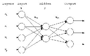
(for input
pattern p). For the other layers, the network input
ℓ+1 to a neuron u ℓ+1 for the input x
ℓ+1 is usually
netpi i pi
computed as follows:
nl
l 1
l l
l 1
net pi
j 1
wij opj i
where Opjℓ = xpi
is the output of the neuron ujℓ of
Fig1 the three layers (input, hidden and output) of
layer ℓ and θi
is the neuron's bias value of
neurons are fully interconnected.
IJSER © 2013 http://www.ijser.org
The research paper published by IJSER journal is about Applying Artificial Neural Network Proton - Proton Collisions at LHC 3
ISSN 2229-5518
To use a NN, it is essential to have some form of training, through which the values of the weights in the network are adjusted to reflect the characteristics of the input data. When the network is trained sufficiently, it will obtain the most nearest correct output for a presented set of input data.
A set of well-defined rules for the solution of a learning problem is called a learning algorithm. No unique learning algorithm exists for the design of NN. Learning algorithms differ from each other in the way in which the adjustment of Δwij to the synaptic weight wij is formulated. In other words, the objective of the learning process is to tune the weights in the network so that the network performs the desired mapping of input to output activation.
NNs are claimed to have the feature of
generalization, through which a trained NN is able
to provide correct output data to a set of
previously (unseen) input data. Training determines the generalization capability in the network structure.
Supervised learning is a class of learning rules for NNs. In which a teaching is provided by telling the network output required for a given input. Weights are adjusted in the learning system so as to minimize the difference between the desired and actual outputs for each input training data. An example of a supervised learning rule is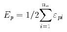
A method, known as “learning by epoch”, first sums gradient information for the whole pattern set and then updates the weights. This method is also known as “batch learning” and most researchers use it for its good performance [25]. Each weight-update tries to minimize the summed error of the pattern set. The error function can be defined for one training pattern pair (xp, dp) as:
Then, the error function can be defined for all the patterns (Known as the Total Sum of Squared, (TSS) errors as: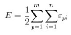
The most desirable condition that we could achieve in any learning algorithm training is εpi ≥0. Obviously, if this condition holds for all patterns in the training set, we can say that the algorithm found a global minimum.
The weights in the network are changed
along a search direction, to drive the weights in the
direction of the estimated minimum. The weight
updating rule for the batch mode is given by:
wijs+1 = Δwijℓ(s) + wijℓ(s)
the delta rule which aims to minimize the error
Where w s+1 is the update weight of w
ijℓ of
function. This means that the actual response of each output neuron, in the network, approaches the desired response for that neuron. This is illustrated in fig. 2.
layer ℓ in the sth learning step, and s is the step
number in the learning process.
In training a network, the available input
data set consists of many facts and is normally
The error εpi for the ith neuron ui
of the
divided into two groups. One group of facts is
output layer o for the training pair (xp, tp) is computed as:
pi t pi opi
This error is used to adjust the weights in such a way that the error is gradually reduced. The training process stops when the error for every training pair is reduced to an acceptable level, or when no further improvement is obtained.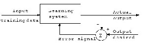
Fig.2. Example of Supervised Learning
used as the training data set and the second group
is retained for checking and testing the accuracy of
the performance of the network after training. The
proposed ANN model was trained using
Levenberg-Marquardt optimization technique [26].
Data collected from experiments are divided into two sets, namely, training set and predicating set. The training set is used to train the ANN model by adjusting the link weights of network model, which should include the data covering the entire experimental space. This means that the training data set has to be fairly large to contain all the required information and must include a wide variety of data from different experimental conditions, including different formulation composition and process parameters.
Linearly, the training error keeps dropping. If the error stops decreasing, or
IJSER © 2013 http://www.ijser.org
The research paper published by IJSER journal is about Applying Artificial Neural Network Proton - Proton Collisions at LHC 4
ISSN 2229-5518
alternatively starts to rise, the ANN model starts to over-fit the data, and at this point, the training must be stopped. In case over-fitting or over- learning occurs during the training process, it is usually advisable to decrease the number of hidden units and/or hidden layers. In contrast, if the network is not sufficiently powerful to model the underlying function, over-learning is not likely to occur, and the training errors will drop to a satisfactory level.
Evolutionary Computation (EC) uses computational models of evolutionary processes based on concepts in biological theory. Varieties of these evolutionary computational models have been proposed and used in many applications, including optimization of NN parameters and searching for new NN learning rules. We will refer to them as Evolutionary Algorithms (EAs) [27-29]
EAs are based on the evolution of a population which evolves according to rules of selection and other operators such as crossover and mutation. Each individual in the population is given a measure of its fitness in the environment. Selection favors individual with high fitness. These individuals are perturbed using the operators. This provides general heuristics for exploration in the environment. This cycle of evaluation, selection, crossover, mutation and survival continues until some termination criterion is met. Although, it is very simple from a biological point of view, these algorithms are sufficiently complex to provide strong and powerful adaptive search mechanisms.
Genetic Algorithms (GAs) were developed in the 70s by John Holland [30], who strongly stressed recombination as the energetic potential of
evolution [32]. The notion of using abstract syntax trees to represent programs in GAs, Genetic Programming (GP), was suggested in [33], first implemented in [34] and popularised in [35-37]. The term Genetic Programming is used to refer to both tree-based GAs and the evolutionary generation of programs [38,39]. Although similar at the highest level, each of the two varieties implements genetic operators in a different manner. This thesis concentrates on the tree-based variety. We will discuss GP further in Section 3.4. In the following two sections, whose descriptions
are mainly based on [30, 32, 33, 35, 36, 37], we give more background information about natural and artificial evolution in general, and on GAs in particular.
As described by Darwin [40], evolution is the process by which populations of organisms gradually adapt over time to enhance their chances of surviving. This is achieved by ensuring that the stronger individuals in the population have a higher chance of reproducing and creating children (offspring).
In artificial evolution, the members of the
population represent possible solutions to a
particular optimization problem. The problem itself represents the environment. We must apply each potential solution to the problem and assign it a fitness value, indicating its performance on the problem. The two essential features of natural evolution which we need to maintain are propagation of more adaptive features to future generations (by applying a selective pressure which gives better solutions a greater opportunity to reproduce) and the heritability of features from parent to children (we need to ensure that the process of reproduction keeps most of the features of the parent solution and yet allows for variety so that new features can be explored) [30].
GAs is powerful search and optimization techniques, based on the mechanics of natural selection [31]. Some basic terms used are:
A phenotype is a possible solution to the
problem;
A chromosome is an encoding representation
of a phenotype in a form that can be used;
A population is the variety of chromosomes
that evolves from generation to generation;
A generation (a population set) represents a
single step toward the solution;
Fitness is the measure of the performance of an
individual on the problem;
Evaluation is the interpretation of the genotype into the phenotype and the computation of its fitness;
Genes are the parts of data which make up a
chromosome.
The advantage of GAs is that they have a consistent structure for different problems. Accordingly, one GA can be used for a variety of
IJSER © 2013 http://www.ijser.org
The research paper published by IJSER journal is about Applying Artificial Neural Network Proton - Proton Collisions at LHC 5
ISSN 2229-5518
optimization problems. GAs is used for a number of different application areas [30]. GA is capable of finding good solutions quickly [32]. Also, the GA is inherently parallel, since a population of potential solutions is maintained.
To solve an optimization problem, a GA requires four components and a termination criterion for the search. The components are: a representation (encoding) of the problem, a fitness evaluation function, a population initialization procedure and a set of genetic operators.
In addition, there are a set of GA control
parameters, predefined to guide the GA, such as
the size of the population, the method by which genetic operators are chosen, the probabilities of each genetic operator being chosen, the choice of methods for implementing probability in selection, the probability of mutation of a gene in a selected individual, the method used to select a crossover point for the recombination operator and the seed value used for the random number generator.
The structure of a typical GA can be described as follows [41]
(1) 0 → t
(2) Population(s) →P(t) (3) Evaluate (P(t))
(4) REPEAT until solution is found
(5) {
(6) t+1→t
(7) Selection (P(t)) →B(t)
(8) Breeding (B(t)) →R(t)
(9) Mutation (R(t)) →M(t) (10) Evaluate M(t)
(11) Survival (M(t), P(t-1)) →P(t) (12) }
Where
S is a random generator seed
t represents the generation
P(t) is the population in generation t
B(t) is the buffer of parents in generation t
R(t) are the children generated by recombining or cloning B(t)
M(t) are the children created by mutating R(t)
In the algorithm, an initial population is generated in line 2. Then, the algorithm computes the fitness for each member of the initial population in line 3. Subsequently, a loop is entered based on whether or not the algorithm's termination criteria are met in line 4. Line 6 contains the control code for the inner loop in which a new generation is created. Lines 7 through 10 contain the part of the algorithm in which new individuals are generated. First, a genetic operator is selected. The particular
numbers of parents for that operator are then selected. The operator is then applied to generate one or more new children. Finally, the new children are added to the new generation.
Lines 11 and 12 serve to close the outer loop of the algorithm. Fitness values are computed for each individual in the new generation. These values are used to guide simulated natural selection in the new generation. The termination criterion is tested and the algorithm is either repeated or terminated.
The most significant differences in GAs are:
GAs search a population of points in parallel, not a single point
GAs do not require derivative information
(unlike gradient descending methods, e.g. SBP) or other additional knowledge - only the objective function and corresponding fitness levels affect the directions of search
GAs use probabilistic transition rules, not deterministic ones
GAs can provide a number of potential solutions to a given problem
GAs operate on fixed length representations.
Genetic connectionism combines genetic search and connectionist computation. GAs have been applied successfully to the problem of designing NNs with supervised learning processes, for evolving the architecture suitable for the problem [42-47]. However, these applications do not address the problem of training neural networks, since they still depend on other training methods to adjust the weights.
GAs have been used for training ANNs either with fixed architectures or in combination with constructive/destructive methods. This can be made by replacing traditional learning algorithms such as gradient-based methods [48]. Not only have GAs been used to perform weight training for supervised learning and for reinforcement learning applications, but they have also been used to select training data and to translate the output behavior of ANNs [49-51]. GAs have been applied to the problem of finding ANN architectures [52-57], where an architecture specification indicates how many hidden units a
IJSER © 2013 http://www.ijser.org
The research paper published by IJSER journal is about Applying Artificial Neural Network Proton - Proton Collisions at LHC 6
ISSN 2229-5518
network should have and how these units should be connected.
The process key in the evolutionary design of neural architectures is shown in Fig 3. The topologies of the network have to be distinct before any training process. The definition of the architecture has great weight on the network performance, the effectiveness and efficiency of the learning process. As discussed in [58], the alternative provided by destructive and constructive techniques is not satisfactory.
The network architecture designing can be
explained as a search in the architecture space that
each point represents a different topology. The
search space is huge, even with a limited number of neurons, and a controlled connectivity. Additionally, the search space makes things even more difficult in some cases. For instance when networks with different topologies may show similar learning and generalization abilities, alternatively, networks with similar structures may have different performances. In addition, the performance evaluation depends on the training method and on the initial conditions (weight initialization) [59]. Building the architectures by means of GAs is strongly reliant on how the features of the network are encoded in the
genotype. Using a bitstring is not essentially the
the weight training and adjusting process, the fitness functions of a neural network can be defined by considering two important factors: the error is the different between target and actual outputs. In this work, we defined the fitness function as the mean square error (SSE).
The approach is to use the GA-ANN
model that is enough intelligent to discover
functions for p-p interactions (mean multiplicity distribution of charged particles with respects of the total center of mass energy). The model is trained/predicated by using experimental data to simulate the p-p interaction.
GA-ANN has the potential to discover a
new model, to show that the data sets are subdivided into two sets (training and predication). GA-ANN discovers a new model by using the training set while the predicated set is used to examine their generalization capabilities.
To measure the error between the experimental data and the simulated data we used the statistic measures. The total deviation of the response values from the fit to the response values. It is also called the summed square of residuals and is usually labeled as SSE. The statistical measures of sum squared error (SSE),
n
SSE ( yi yˆ i )
best approach to evolve the architecture. Therefore,
a determination has to be made concerning how
the information about the architecture should be
where
i 1
yˆi
2
is the predicted value for xi
encoded in the genotype.
To find good ANN architectures using
GAs, we should know how to encode architectures
and
yi is the observed data value occurring at xi .
The proposed GA-ANN hybrid model has
(neurons, layers, and connections) in the chromosomes that can be manipulated by the GA. Encoding of ANNs onto a chromosome can take many different forms.
This study proposed a hybrid model combined of ANN and GA (We called it “GA– ANN hybrid model”) for optimization of the weights of feed-forward neural networks to improve the effectiveness of the ANN model. Assuming that the structure of these networks has been decided. Genetic algorithm is run to have the optimal parameters of the architectures, weights and biases of all the neurons which are joined to create vectors.
We construct a genetic algorithm, which
can search for the global optimum of the number of hidden units and the connection structure between the inputs and the output layers. During
been used to model the multiplicity distribution of
the charged shower particles. The proposed model
was trained using Levenberg-Marquardt![]()
optimization technique [26]. The architecture of GA-ANN has three inputs and one output. The inputs are the charged particles multiplicity (n), the total center of mass energy ( s ), and the pseudo rapidity ().The output is the charged particles multiplicity distribution (Pn). Figure 3 shows the schematic of GA-ANN model.
Data collected from experiments are
divided into two sets, namely, training set and predicating set. The training set is used to train the GA- ANN hybrid model. The predicating data set is used to confirm the accuracy of the proposed model. It ensures that the relationship between inputs and outputs, based on the training and t predicating sets are real. The data set is divided into two groups 80% for training and 20% for predicating. For work completeness, the final
IJSER © 2013 http://www.ijser.org
The research paper published by IJSER journal is about Applying Artificial Neural Network Proton - Proton Collisions at LHC 7
ISSN 2229-5518
weights and biases after training are given in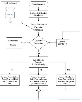
Appendix A.
A
model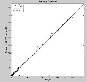
Figure 3: Overview of GA-ANN hybrid
The input patterns of the designed GA- ANN hybrid have been trained to produce target patterns that modeling the pseudo-rapidity distribution. GAs parameters are adjusted as in table 1. The fast Levenberg-Marquardt algorithm (LMA) has been employed to train the ANN. In order to obtain the optimal structure of ANN, we have used GA as hybrid model.
Table 1. GA parameters for modelling ANN.
B
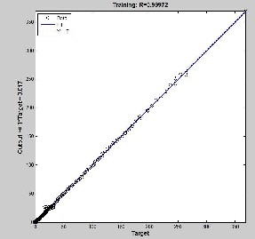
Figure 4: A is the regression values between the target and the training well, B is the regression values between the target and the predication![]()
Simulation results based on both ANN and GA-ANN hybrid model, to model the distribution of shower charged particle produced for P-P at different the total center of mass energy,
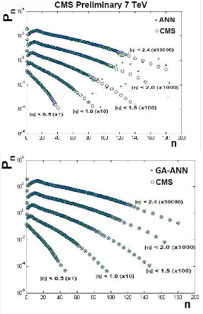
s 0.9 TeV, 2.36 TeV and 7 TeV, are given in Figure 5, 6, and 7 respectively. We notice that the curves obtained by the trained GA-ANN hybrid model show an exact fitting to the experimental data in the three cases.
Figure 4 shows that the GA-ANN model
succeeds to learn/predicate the training/
IJSER © 2013 http://www.ijser.org
The research paper published by IJSER journal is about Applying Artificial Neural Network Proton - Proton Collisions at LHC 8
ISSN 2229-5518
predicating set respectively. Where, R is the regression values for each of the raining set matrix.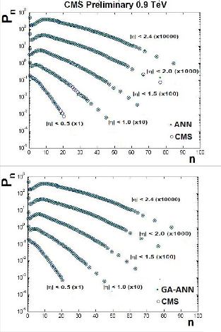
![]()
Figure 5: ANN and GA-ANN simulation results for charge particle Multiplicity distribution of shower p-p at s =0.9 TeV
Then, the GA-ANN Hybrid model is able to exactly model for the charge particle multiplicity distribution. The total sum of squared error SSE, the weights and biases which used for the designed network is provided in the Appendix A.
In this model we have obtained the minimum error (=0.0001) by using GA. Table 2 shows a comparison between the ANN model and the GA-ANN model for the prediction of the pseudo-rapidity distribution. In the 3x15x15x1
ANN structure, we have used 285 connections and
obtained an error equal to 0.0001, while the connection in GA-ANN model is 225. Therefore,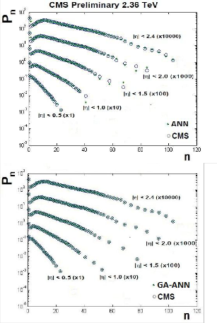
we noticed in the ANN model that by increasing the number of connections to 285 the error decreases to 0.01, but this needs more calculations. By using GA optimization search, we have obtained the structure which minimizes the number of connections equals to 229 only and the error (= 0.0001). This indicates that the GA-ANN hybrid model is more efficient than the ANN model.![]()
Figure 6: ANN and GA-ANN simulation results for charge particle Multiplicity distribution of shower p-p at s =2.36 TeV
Table 2: Comparison between the different training algorithms (ANN and GA-ANN) for the for charge particle Multiplicity distribution.
IJSER © 2013 http://www.ijser.org
The research paper published by IJSER journal is about Applying Artificial Neural Network Proton - Proton Collisions at LHC 9
ISSN 2229-5518
The efficient ANN structure is given as follows: [3x15x15x1] or [ixjxkxm].
Weights coefficient after training are:
Wji = [3.5001 -1.0299 1.6118
0.7565 -2.2408 3.2605
-1.4374 1.1033 -3.1349
2.0116 2.8137 -1.7322
-3.6012 -1.5717 -0.2805
-1.6741 -2.5844 2.7109
-2.0600 -3.1519 1.2488
-0.1986 1.0028 -4.0855
2.6272 0.8254 3.6292
-2.3420 3.0259 -1.9551
-3.2561 0.4683 3.0896
1.2442 -0.8996 -3.4896
-3.2589 -1.1887 2.0875
-1.0889 -1.2080 4.3688
-2.7820 -1.4291 2.3577
3.1861 -0.6309 2.0691
3.4979 0.2456 -2.6633
-0.4889 2.4145 -2.8041
2.1091 -0.1359 -3.4762
-0.1010 4.1758 -0.2120
3.5538 -1.5615 -1.4795
-3.4153 1.2517 2.1415
2.6232 -3.0757 0.0831
1.7632 1.9749 -2.5519
7.6987 0.0526 0.4267![]()
Figure 7: ANN and GA-ANN simulation results for charge particle Multiplicity distribution of shower p-p at s =7 TeV
![]()
The paper presents the GA-ANN as a new technique for constructing the functions of the multiplicity distribution of charged particles, Pn (n,![]()
, s ) of p-p interaction. The discovered models show good match to the experimental data. Moreover, they are capable of predicating experimental data for Pn (n, , s ) that are not
used in the training session.![]()
Consequence, the predicating values of Pn (n, , s ) in terms of the same parameters are in good agreement with the experimental data from
Particle Data Group. Finally, we conclude that
GA-ANN has become one of important research
areas in the field of high Energy physics.
].
Wkj = [-0.3294 -0.5006 0.0421 0.3603 0.5147
0.5506 -0.2498 -0.2678 0.2670 -0.3568
-0.3951 0.2529 -0.2169 0.4323 0.0683
0.1875 -0.2948 0.2705 0.2209 0.1928
-0.2207 -0.6121 -0.0693 -0.0125 0.4214
-0.4698 -0.0697 -0.4795 0.0425 0.2387
0.1975 -0.1441 0.2947 -0.1347 -0.0403
-0.0745 0.2345 0.1572 -0.2792 0.3784
0.1043 0.4784 -0.2899 0.2012 -0.4270
0.5578 -0.7176 0.3619 0.2601 -0.2738
-0.1081 -0.2412 0.0074 -0.3967 -0.2235
0.0466 -0.0407 0.0592 0.3128 -0.1570
0.4321 0.4505 0.0313 -0.5976 -0.0851
-0.4295 -0.4887 0.0694 -0.3939 -0.0354
-0.1972 -0.1416 0.1706 -0.1719 -0.0761
0.2102 0.0185 -0.1658 -0.1943 -0.4253
0.2685 0.4724 0.4946 -0.3538 0.1559
0.3198 0.1207 0.5657 -0.3894 0.1497
-0.5528 0.4031 0.5570 0.4562 -0.5802
0.3498 -0.3870 0.2453 0.4581 0.2430
0.2047 -0.0802 0.1584 0.2806 -0.2790
0.0981 -0.5055 0.2559 -0.0297 -0.2058
IJSER © 2013 http://www.ijser.org
The research paper published by IJSER journal is about Applying Artificial Neural Network Proton - Proton Collisions at LHC 10
ISSN 2229-5518
-0.3498 -0.5513 0.0022 -0.3034 0.2156
-0.6226 -0.4085 0.4338 -0.0441 -0.4801
-0.0093 0.0875 0.0815 0.3935 0.1840
0.0063 0.2790 0.7558 0.3383 0.5882
-0.5506 -0.0518 0.5625 0.2459 -0.0612
0.0036 0.4404 -0.3268 -0.5626 -0.2253
0.5591 -0.2797 -0.0408 0.1302 -0.4361
-0.6123 0.4833 -0.0457 0.3927 -0.3694
-0.0746 -0.0978 0.0710 -0.7610 0.1412
-0.3373 0.4167 0.3421 -0.0577 0.2109
0.2422 0.2013 -0.1384 -0.3700 -0.4464
0.0868 -0.5964 -0.0837 -0.7971 -0.4299
-0.6500 -1.1315 -0.4557 1.6169 -0.3205
0.2205 1.0185 0.4752 -0.4155 0.1614
1.2311 0.0061 -0.0539 0.6813 0.9395
-0.4295 -0.3083 0.2768 -0.1151 0.0802
-0.6988 0.2346 -0.3455 0.0432 0.1663
-0.0601 0.0527 0.3519 0.3520 -0.7821
-0.6241 -0.1201 -0.4317 0.7441 0.7305
0.5433 -0.6909 0.4848 -0.3888 0.3710
-0.6920 -0.0190 -0.4892 0.1678 0.0808
-0.3752 -0.1745 -0.7304 0.0462 -0.3883
].
Wmk = [0.9283 1.6321 0.0356 -0.4147 -0.8312
-3.0722 -1.9368 1.7113 0.0100 -0.4066
0.0721 0.1362 0.4692 -0.9749 1.7950].
bi = [-4.7175 -2.2157 3.6932 ].
bj = [-4.1756 -3.8559 3.9766 -3.3430 2.7598 2.5040
2.1326 1.9297 -0.6547 0.7272 0.5859 -1.1575
0.3029 0.3486 -0.4088].
bk = [ 1.7214 -1.7100 1.5000 -1.2915 1.1448
1.0033 -0.6584 -0.4397 -0.4963 -0.3211
0.2594 -0.1649 0.0603 -0.1078]. bm = [-0.2071].
The authors highly acknowledge and deeply appreciate the supports of the Egyptian Academy of Scientific Research and Technology (ASRT) and the Egyptian Network for High Energy Physics (ENHEP).
1) CMS Collaboration, J. High Energy Phys. 01 079(2011).
2) CMS Collaboration, J. High Energy Phys. 08 141(2011).
3) CMS Collaboration, Phys. Rev. Lett. 105 022002(2010).
4) ATLAS Collaboration, Phys. Lett. B 707 330-348(2012).
5) ATLAS Collaboration, Phys. Lett. B, 2011.
6) ALICE Collaboration, Phys. Lett. B 693 53-68(2010).
7) ALICE Collaboration, Eur. Phys. J. C 68345-354 (2010).
8) TOTEM Collaboration, EPL 96 21002(2011).
9) M. Jacob, R. Slansky, Phys. Rev. D 5, 1847 (1972)
10) R. Hwa, Phys. Rev. D 1, 1790 (1970)
11) R. Hwa, Phys. Rev. Lett. 26, 1143 (1971)
12) R. Engel, Z. Phys. C 66 (1995) 203; R. Engel, J. Ranft and
S. Roesler, Phys. Rev. D 52 (1995).
13) L. Teodorescu, D. Sherwood, Comput. Phys. Commun.
178, 409 (2008)
14) L. Teodorescu, IEEE T. Nucl. Sci. 53, 2221 (2006)
15) J.M. Link, Nucl. Instrum. Meth. A 551, 504 (2005)
16) S. Yaseen El-Bakry, Amr Radi, Int. J. Mod. Phys. C 18,
351 (2007)
17) E. El-dahshan, A. Radi, M.Y. El-Bakry, Int. J. Mod.
Phys. C 20, 1817 (2009)
18) S. Whiteson, D. Whiteson, Eng. Appl. Artif. Intel. 22,
1203 (2009)
19) S. Haykin, Neural networks a comprehensive foundation
(2nd ed.), Prentice Hall (1999).
20) J.H. Holland, Adaptation in Natural and Artificial
Systems (University of Michigan Press, Ann Arbo r,
1975)
21) J.R. Koza, Genetic Programming: On the Programming
of Computers by means of Natural Selection (The MIT Press, Cambridge, MA, 1992)
22) Ferreira, C., Gene Expression Programming: Mathematical Modeling by an Artificial Intelligence, 2nd Edition, Springer-Verlag Germany2006.
23) A.E. Eiben, J.E. Smith, Introduction to Evolutionary
Algorithms (Springer, Berlin, 2003)
24) Amr Radi, Discovery of Neural network learning rules using genetic programming. PHD, the School of computers Sciences, Birmingham University, 2000.
25) L Teodorescu., High energy physics data analysis with
gene expression programming. In 2005 IEEE Nuclear
Science Symposium Conference Record, Vol. 1, pp. 143-
147, 2005.
26) M.T. Hagan and M.B. Menhaj, "Training feedforward networks with the Marquardt algorithm", IEEE Transactions on Neural Networks, Vol 6, pp 861-867,
1994.
27) T. Back, Evolutionary Algorithms in Theory and
Practice, Oxford University Press, New York, 1996.
28) D. B. Fogel (1994) "An Introduction to
Simulated Evolutionary Optimization," IEEE Trans.
29) Neural Networks, Vol. 5:1, pp. 3-14.
30) T. Back, U. Hammel, and H.-P. Schwefel (1997)
"Evolutionary Computation: Comments on
31) the History and Current State," IEEE
Trans. Evolutionary Computation, Vol. 1:1, pp. 3-17.
32) . H. Holland. Adaptation in Natural and Artificial
Systems. The University of Michigan Press, Ann Arbor, Michigan, 1975.
33) Fogel DB (1995) Evolutionary Computation: Toward a
New Philosophy of Machine Intelligence, IEEE Press, Piscataway, NJ.
34) D. E. Goldberg, Genetic Algorithm in Search Optimization and Machine Learning(Addison-Wesley, New York, 1989).
35) Richard Forsyth. Richard Forsyth. BEAGLE A
Darwinian Approach to Pattern Recognition.
Kybernetes, 10(3):159-166, 1981.
36) Cramer, Nichael Lynn (1985), "A representation for the
Adaptive Generation of Simple Sequential Programs" in Proceedings of an International Conference on
IJSER © 2013 http://www.ijser.org
The research paper published by IJSER journal is about Applying Artificial Neural Network Proton - Proton Collisions at LHC 11
ISSN 2229-5518
Genetic Algorithms and the Applications, Grefenstette, John J. (ed.), CMU
37) Koza, J.R. (1992), Genetic Programming: On the Programming of Computers by Means of Natural Selection, MIT Press
38) Koza, J.R. (1994), Genetic Programming II: Automatic
Discovery of Reusable Programs, MIT Press
39) Koza, J.R., Bennett, F.H., Andre, D., and Keane, M.A.
(1999), Genetic Programming III: Darwinian Invention
and Problem Solving, Morgan Kaufmann
40) Banzhaf, W., P. Nordin, R. E. Keller, and F. D.
Francone, 1998. Genetic Programming: An Introduction: On the Automatic Evolution of Computer Programs and its Applications, Morgan Kaufmann.
41) Mitchell, M., 1996. An Introduction to Genetic
Algorithms, MIT Press.
42) Darwin, C 1959. The Autobiography of Charles Darwin: With original omissions restored, edited with appendix and notes by his grand-daughter, Nora Barlow, Norton.
43) Darrel Whitley, “A genetic algorithm tutorial”,
Statistics and Computing (1994) 4, 65-85.
44) A new algorithm for developing dynamic radial basis function neural network models based on genetic algorithms
45) H Sarimveis, A Alexandridis, S Mazarkakis, G Bafas
in Computers & Chemical Engineering (2004)
46) An optimizing BP neural network algorithm based on
genetic algorithm
47) Ding Shifei, Su Chunyang in Artificial Intelligence
Review (2010)
48) Hierarchical genetic algorithm based neural network design
49) G G Yen, H Lu in IEEE Symposium on Combinations of Evolutionary Computation and Neural Networks (2000)
50) Genetic Algorithm based Selective Neural Network
Ensemble
51) Z H Zhou, J X Wu, Y Jiang, S F Chen in Proceedings of the 17th International Joint Conference on Artificial Intelligence (2001)
52) Modified backpropagation algorithms for training the multilayer feedforward neural networks with hard- limiting neurons
53) Xiangui Yu, N K Loh, GA Jullien, WC Miller
in Proceedings of Canadian Conference on Electrical and Computer Engineering (1993)
54) Training Feedforward Neural Networks Using Genetic
Algorithms
55) David J Montana, Lawrence Davis in Machine
Learning (1989)
56) A.J.F. van Rooij; L.C. Jain and R.P. Johnson, Neural
network training using genetic algorithms. (Singapore: World Scientific, 1996).
57) Maniezzo, 1994): Vittorio Maniezzo: “Genetic Evolution
of the Topology and
58) Weight Distribution of Neural Networks”, in: IEEE
Transactions of Neural
59) Networks, Vol. 5, No. 1, pp 39-53
60) Bornholdt, 1992): Stefan Bornholdt and Dirk Graudenz:
“General Asymmet-
61) ric Neural Networks and Structure Design by Genetic
Algorithms”, in:
62) Neural Networks, Vol. 5, pp. 327-334, Pergamon Press
63) Kitano, 1990a): Hiroaki Kitano: “Designing Neural
Networks Using Genetic
64) Algorithms with Graph Generation Systems”,
in: Complex Systems, No. 4,
65) p. 461-476
66) NOLFI, S., & Parisi, D. (1994) 'Desired answers do not
correspond to good teaching inputs in ecological neural networks', Neural processing letters, Vol. 1(2), p. 1-4.
67) NOLFI, S., & Parisi, D. (1996) 'Learning to adapt to changing environments in evolving neural networks', Adaptive Behavior, Vol. 5(1), pp. 75-97.
68) NOLFI, S., Parisi, D., & Elman, J. L. (1994) 'Learning and evolution in neural networks', Adaptive Behavior,
3(1), pp. 5-28.
69) PUJOL, J. C. F., & Poli, R. (1998) 'Efficient evolution of
asymmetric recurrent neural networks using a two-
dimensional representation', Proceedings of the first European workshop on genetic programming (EUROGP) , pp. 130-141.
70) MILLER, G. F., Todd, P. M., & Hedge, S. U. (1989),
'Designing neural networks using genetic algorithms', Proceedings of the third international conference on genetic algorithms and their applications, pp. 379-384.
71) MANDISCHER, M. (1993) 'Representation and
evolution of neural networks', Artificial neural nets and genetic algorithms proceedings of the international conference at Innsbruck, Austria, pp. 643-649. Wien and New York: Springer.
72) Joao Carlos Figueira Pujol. Evolution of Artificial
Neural Networks Using a Two-dimensional Representation. PhD thesis, School of Computer Science, University of Birmingham, UK, 1999.
73) X. Yao (1995f), ``Evolutionary artificial neural
networks,'' In Encyclopedia of Computer Science and Technology, Vol.33, ed. A. Kent and J. G. Williams, Marcel Dekker Inc., New York. pp.137-170. Also appearing in Encyclopedia of Library and Information Science.
IJSER © 2013 http://www.ijser.org