International Journal of Scientific & Engineering Research, Volume 4, Issue 9, September-2013 2105

ISSN 2229-5518

Analysis of Vibrations of Automobile Suspension System Using

Full-car Model

A. Bala Raju1 and R. Venkatachalam2

ABSTRACT

The suspension system of an automobile helps to support the car body, engine and passengers, and at the same time absorbs shocks received from the ground while vehicle moves on rough roads. The study of vibrations of the suspension system has been a topic of interest to many researchers in the past. Most of them have studied using quarter car model and half car model. These models represent the original system in an approximate way. Very few people have been working on full car model. Most of the literature presents the final results. The equations of motion together with development is missing in the literature, may be because of confidential nature of the work. Hence, in this paper it is aimed at deriving the equations of motion and study the vibrations of the suspension system under different disturbing conditions. The responses obtained are in close agreement with results present in the literature.

Key words: Suspension System, Response, Disturbing inputs, Equations of motion

1. INTRODUCTION

The vehicle suspension forms one very
important system for an automobile. This is the one which helps to support the engine, vehicle body and passengers and at the same time absorbs the shocks arising due to roughness of the road.
The usual arrangement consists of supporting the chassis through springs and dampers, by the axle. The engine and the body of the vehicle are attached to the chassis rigidly. Hence, the chassis along with the body of the vehicle, engine and the passengers may be considered to be one unit only. The springs and dampers which connect the axle and chassis play an important role in absorbing shocks and keeping chassis affected to a minimum level.

The review of the past literature reveals that this has been a subject of interest to many researchers. Attempts have been made to perform the studies on quarter car model and half car model of the vehicle, which are shown in Figure 1.

(a) (b)

Figure 1 The models including the effect of pneumatic tyres (a) Quarter car model (b) Half car model

These models represent the original system, in an
approximate and simplified manner. However, they are not realistic models.

1 Research Scholar, Mechanical Engineering Department, National Institute of Technology, Warangal,

Email: baluap2002@ya hoo.co.in

2 Professor of Mechanical Engineering, National Institute of

Technology, Warangal, Email: chalamrv@yahoo.com.

Many of the past researchers have concentrated on quarter car models and half car models. The research works of Hedrick [1], Gobbi [2], Ahmed Fahem [3], are some of the works based on quarter car model. Hedrick[1] considered a quarter car model with hydraulic actuator acting under the effect of coulomb friction. An absorber based nonlinear controller and adaptive nonlinear controller are proposed. Employing two sensors, one for displacement and other for velocity measurements, Gobbi [2], Wei Gao et al. [6] studied dynamic behaviour of passively suspended vehicles running on rough roads. The road profile is considered to give random inputs to the suspension system. Ahmed Faheem [3] studied the dynamic behaviour using quarter car model and half car model for different excitations given by the road. Jacquelien et al. [4] used electrical analogy in conjunction with quarter car model and studied the control scheme of the suspension system. Wei Gao et al. [5] also studied the dynamic characteristics considering the mass, damping and tyre stiffness as random variables. Kamalakannan et al. [6] tried adaptive control by varying damping properties according to the road conditions. Sawant et al.[7]developed an experimental procedure for determining the suspension parameters using a quarter car model. Thite [8] refined the quarter car model to include the effect of series stiffness. State space equations are employed to calculate the natural frequency and model damping ratios. Gadhia et al. [9] analysed quarter car model for rear suspension using ADAMS software.
Lin [10], Husiyno [11] , Li-Xing Gao [12], Thite [13] ,
Roberto Barbosa [14],performed studies using half car models. Lin [10] performed a time domain direct identification for vehicle mass, damping and stiffness. Husiyno [11] studied multi objective control of half car suspension system. It is observed that when the tyre damping coefficients are precisely estimated, the road holding quality of the suspension system can be improved to some extent. Li-Xing Gao [12] considered a half car model in conjunction with pseudoexcitation for the road conditions and studied
the dynamic response of the vehicle. Thite et al. [13]

International Journal of Scientific & Engineering Research, Volume 4, Issue 9, September-2013 2106

ISSN 2229-5518

used a frequency domain method for estimating suspension system parameters. Roberto Barbosa [14] studied the frequency response of half car model due to pavement roughness. The quarter car model and half car model represent the actual car in an approximate way. An automobile, in principle can exhibit three rotations, roll, yaw and pitch, in addition to up and down vertical linear motion and linear motion in the horizontal plane. In total, it can have three displacements and three rotations. However, due to stiffness in the suspension system, the two components of displacements in the horizontal plane and yaw motion may be ignored totally. Any disturbance due to roughness of the road naturally effects up and down linear motion and, roll and pitch rotations. The quarter car model cannot consider roll and pitch motion. A half car model can consider either roll motion or pitch motion, depending on whether it is roll bounce model or pitch bounce model. The coupling of motions cannot be seen in these models. That is way these models cannot be realistic. However, they form a quick and good initial start to the actual problem. Attempts are also being made to analyze the four wheeler as it is. Libin Li [15] performed computer simulation studies through multi body model, identifying twenty degrees of freedom. Pater Gaspar [16] considered full car model and proposed a method for identifying suspension parameters taking in to account nonlinear nature of the components. Anil Shirahatt et al.[17] attempted to maximize the comfort level considering a full car model. Genetic algorithms have been employed to perform optimization to arrive at optimum values of suspension parameters. Hajkurami et al. [18] studied the frequency response of a full car model as a system of seven degrees of freedom. Ikbal Eski [19] obtained neural network base control system for full car model. Guidaa et al. [20] proposed a method of identifying parameter of a full car model. The analysis has been developed for designing an active suspension system. Kasi Kamalakkannan et al. [21] performed studies on design, modelling, simulation and testing procedure for All Terrain Vehicles.
Though lot of work has been presented in the literature, the basic development of Equations is not been disclosed. In almost all the papers, only some of the final results are presented through graphs. It is then felt that one must clearly explain the development of basic equations which will be very useful for those who will be interested in pursuing research work in the area of vehicle suspension system. Therefore, in this paper it is attempted to present the development of equations of motion for a full car model. This may not be anything new to the people already working this area. But this will be useful to researchers entering into this area because one can make interpretation to the results only when development of equations is clear.

Nomenclature

2. Description of the Model

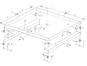
Figure 2 shows a mass m3 being supported at its four corners. The mass m3 includes mass of the chassis, engine, automobile body and passengers. The masses m1 and m2 are, respectively, masses of the front wheel axle and the rear wheel axle. m1 and m2 may also be considered to have included the masses of tyres. k1 and c1 represent the stiffness and damping properties of each of the tyres. k2 and c2 may represent the stiffness and damping of the supporting springs and damper at the front wheels. Similarly, k3 and c3 represent the springs and damper at the rear wheels. Seven coordinates are chosen to describe the motion of the entire system.

Figure 2 Full car model, 7 degrees of freedom

The vertical linear motion of the centre of mass G1 of the front axle and its roll motion may be represented, respectively, by x1 and γ1 . Similarly, x2 and γ2 may describe the linear vertical motion of the centre of mass G2 and the roll motion of the rear axle. The vertical motion of the centre of mass G3 of the mass m3 may be described by the coordinate x3 . The roll and pitch motions of the mass m3 may be described, respectively, by γ and λ. The seven coordinates which describe the vibrating system are, x1 , x2 , x3 , γ1 , γ2 , γ and λ. The vertical displacements caused by the road roughness may be represented by the variables y1 , y2 , y3 and y4 , as shown in the Figure 3. These displacements are to be considered as inputs to the system.

International Journal of Scientific & Engineering Research, Volume 4, Issue 9, September-2013 2107

ISSN 2229-5518

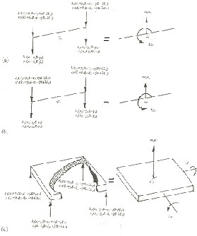
Giving positive displacements to each of the coordinates, the free body diagrams may be draw as shown in Figure 3, and the equations of motion may be obtained as,

Figure 3 Free body diagrams

to be observed from Equations (2 and 4) that the roll motions of the axles are influenced by difference of spring forces and difference of damping forces. It is further to be observed that γ1 , γ2 and γ are neither influencing nor influenced by x1 , x2 , x3 and λ. This is a consequence of the way the coordinates are selected for describing the motion. Now the total seven variables may be split up into two groups; (x1 , x2 , x3 and λ) as one group and (γ1 , γ2 and γ) as another group. The inputs are influencing both the groups.
Renaming the coordinates asX1 = x1 , X2 = x2 , X3 = x3 , X4 = λ , X5 = γ1 , X6 = γ2 and X7 = γ, the equations of motions (1) to (7) may be represented in matrix form as,
𝑴𝑿� + 𝑪𝑿� + 𝑲𝑿� = 𝑭� (8)
where, M , C and K are mass, damping and stiffness
matrices, each of size (7×7). These matrices have nonzero elements in (4×4) space at the top left corner and in (3×3) space at the bottom right corner. This shows that the system of seven differential equations may be split up into two groups as
where the mass, damping and stiffness matrices of the two groups may be expressed as

𝒎𝟏 𝟎 𝟎 𝟎

𝒎𝟏𝒙𝟏 + 𝟐(𝒌𝟏 + 𝒌𝟐)𝒙𝟏 − (𝟐𝒌𝟐 )𝒙𝟑 − (𝟐𝒌𝟐 𝑳𝟏) + 𝟐(𝒄𝟏 + 𝒄𝟐)𝒙𝟏 −

(1)

𝟎 𝒎𝟐 𝟎 𝟎

(𝟐𝒄𝟐)𝒙𝟑 − (𝟐𝒄𝟐𝑳𝟏)𝝀 = 𝒌𝟏(𝒚𝟏 + 𝒚𝟐) + 𝒄𝟏(𝒚𝟏 + 𝒚𝟐 ) (1)

𝑰𝟏 𝜸𝟏 + 𝟐( 𝒌𝟏 + 𝒌𝟐 )𝑩𝟐 𝜸𝟏 − (𝟐𝒌𝟐 𝑩𝟐 )𝜸 +𝟐(𝒄𝟏 + 𝒄𝟐 )𝑩𝟐 𝜸𝟏

−(𝟐𝒄𝟐 𝑩𝟐 )𝜸 = −𝒌𝟏 𝑩(𝒚𝟏 − 𝒚𝟐 ) − 𝒄𝟏 𝑩(𝒚𝟏 − 𝒚𝟐 )

M = � 𝟎 𝟎

𝟎 𝟎

𝒎𝟑

𝟎

𝟎 � (10)

𝑰𝟒

(2)

𝒎𝟐𝒙𝟐 + 𝟐(𝒌𝟏 + 𝒌𝟑)𝒙𝟐 − (𝟐𝒌𝟑 )𝒙𝟑 + (𝟐𝒌𝟑 𝑳𝟐)𝝀 + 𝟐(𝒄𝟏 + 𝒄𝟑)𝒙𝟐

⎡

𝑪(𝟏) = ⎢

𝟐(𝒄𝟏 + 𝒄𝟐 ) 𝟎 −𝟐𝒄𝟐 −𝟐𝒄𝟐 𝑳𝟏 ⎤

𝟎 𝟐(𝒄𝟏 + 𝒄𝟑 ) −𝟐𝒄𝟑 𝟐𝒄𝟑 𝑳𝟐 ⎥

⎢ −𝟐𝒄𝟐

−𝟐𝒄𝟑

𝟐(𝒄𝟐 + 𝒄𝟑 )

𝟐(𝒄𝟐 𝑳𝟏 − 𝒄𝟑 𝑳𝟐 ) ⎥

−(𝟐𝒄𝟑)𝒙𝟑 + (𝟐𝒄𝟑𝑳𝟐)𝝀 = 𝒌𝟏(𝒚𝟑 + 𝒚𝟒) + 𝒄𝟏(𝒚𝟑+ 𝒚𝟒) (3)

⎣ −𝟐𝒄𝟐 𝑳𝟏

𝟐𝒄𝟑 𝑳𝟐

𝟐(𝒄𝟐 𝑳𝟏 − 𝒄𝟑 𝑳𝟐 )

𝟐(𝒄𝟐 𝑳𝟏

𝟑 𝟐

𝑰𝟐 𝜸𝟐 + 𝟐( 𝒌𝟏 + 𝒌𝟑 )𝑩𝟐𝜸𝟐 − (𝟐𝒌𝟑𝑩𝟐)𝜸 +𝟐(𝒄𝟏 + 𝒄𝟑)𝑩𝟐𝜸𝟐

−(𝟐𝒄𝟑𝑩𝟐 )𝜸 = −𝒌𝟏𝑩(𝒚𝟑 − 𝒚𝟒) − 𝒄𝟏𝑩(𝒚𝟑− 𝒚𝟒) (4)

𝒎𝟑𝒙𝟑 − (𝟐𝒌𝟐)𝒙𝟏 − (𝟐𝒌𝟑)𝒙𝟐 + 𝟐(𝒌𝟐 + 𝒌𝟑 )𝒙𝟑 +

𝟐 + 𝒄 𝑳𝟐 ) ⎦

⎡ 𝟐(𝒌𝟏 + 𝒌𝟐 ) 𝟎 −𝟐𝒌𝟐 −𝟐𝒌𝟐 𝑳𝟏 ⎤

𝑲(𝟏) = ⎢ 𝟎 𝟐(𝒌𝟏 + 𝒌𝟑 ) −𝟐𝒌𝟑 𝟐𝒌𝟑 𝑳𝟐 ⎥

𝟐(𝒌𝟐𝑳𝟏 − 𝒌𝟑𝑳𝟐)𝝀 − (𝟐𝒄𝟐)𝒙𝟏 − (𝟐𝒄𝟑)𝒙𝟐 +

⎢ −𝟐𝒌𝟐

⎣ −𝟐𝒌 𝑳

−𝟐𝒌𝟑

𝟐𝒌 𝑳

𝟐(𝒌𝟐 + 𝒌𝟑 )

𝟐(𝒌 𝑳 − 𝒌 𝑳 )

𝟐(𝒌𝟐 𝑳𝟏 − 𝒌𝟑 𝑳𝟐 ) ⎥

𝟐(𝒌 𝑳𝟐 + 𝒌 𝑳𝟐 ) ⎦

𝟐(𝒄𝟐 + 𝒄𝟑)𝒙𝟑 + 𝟐(𝒄𝟐𝑳𝟏 − 𝒄𝟑𝑳𝟐 )𝝀 = 0 (5)

𝟐 𝟏

𝟑 𝟐

𝟐 𝟏

𝟑 𝟐

𝟐 𝟏

𝟑 𝟐

𝑰𝟑 𝜸 − (𝟐𝒌𝟐𝑩𝟐)𝜸𝟏 − (𝟐𝒌𝟑 𝑩𝟐)𝜸𝟐 + 𝟐(𝒌𝟐 + 𝒌𝟑 )𝑩𝟐𝜸

−(𝟐𝒄𝟐𝑩𝟐)𝜸𝟏 − (𝟐𝒄𝟑𝑩𝟐)𝜸𝟐 + 𝟐(𝒄𝟐 + 𝒄𝟑)𝑩𝟐𝜸 = 𝟎 (6)

𝑰𝟒 𝝀 − (𝟐𝒌𝟐𝑳𝟏)𝒙𝟏 + (𝟐𝒌𝟑𝑳𝟐)𝒙𝟐 + 𝟐(𝒌𝟐 𝑳𝟏 − 𝒌𝟑 𝑳𝟐)𝒙𝟑 +

𝟐(𝒌𝟐𝑳𝟐 +)λ−(𝟐𝒄 𝑳 )𝒙 + (𝟐𝒄 𝑳 )𝒙 +

X (1) = [ 𝒙𝟏

(1)

𝒙𝟐
𝒙𝟑

(11,12)

𝝀 ]𝑇 (13)

𝟐 𝟐

(𝒚
+ 𝒚 ) + 𝒄 (𝒚
+ 𝒚 ) ⋮

𝟐(𝒄𝟐𝑳𝟏 − 𝒄𝟑𝑳𝟐)𝒙𝟑 + 𝟐(𝒄𝟐𝑳𝟏 + 𝒄𝟑𝑳𝟐)𝝀 = 0 (7)

F = { 𝒌𝟏 𝟏 𝟐

𝟏 𝟏 𝟐

The motion of the entire suspension system may be
described by the Equations (1) to (7). These are forming a set of seven second order, linear, ordinary
differential equations. The roughness of the road is
𝒌𝟏 (𝒚𝟑 + 𝒚𝟒 ) + 𝒄𝟏 (𝒚𝟑 + 𝒚𝟒 ) ⋮ 0 ⋮ 0 }
𝑰𝟏 𝟎 𝟎

M (2) = � 𝟎 𝑰𝟐 𝟎 �

𝟎 𝟎 𝑰
(14)
(15)

providing inputs to the system through 𝒚𝐢 and 𝒚𝒊 , i = 𝟑

1 to 4. These inputs are effecting only the

𝟐(𝒄𝟏 + 𝒄𝟐 )𝑩𝟐 𝟎 −𝟐𝒄𝟐 𝑩𝟐

displacements (x1 and x2 ) and roll motions (γ1 and γ2 )
of the axles. This is because the axles are the first ones
to get influenced by the roughness of the road,

C (2) = �

𝟎 𝟐(𝒄𝟏 + 𝒄𝟑 )𝑩𝟐 −𝟐𝒄𝟑 𝑩𝟐 �

−𝟐𝒄𝟐 𝑩𝟐 −𝟐𝒄𝟑 𝑩𝟐 𝟐(𝒄𝟐 + 𝒄𝟑 )𝑩𝟐

𝟐(𝒌𝟏 + 𝒌𝟐 )𝑩𝟐 𝟎 −𝟐𝒌𝟐 𝑩𝟐

through the tyres. The motions of the axles in turn

(2) �

𝟎 𝟐(𝒌

+ 𝒌 )𝑩𝟐 −𝟐𝒌 𝑩𝟐 �

effect the vertical motion (x3 ) , roll motion (γ) and K =

𝟏 𝟑 𝟑

𝟐 𝟐 𝟐

pitch motion (λ) of mass m3 . The inputs 𝒚𝒊 and 𝒚𝒊
are not influencing x3 , γ and λ directly. It is to be

−𝟐𝒌𝟐 𝑩

−𝟐𝒌𝟑 𝑩

𝟐(𝒌𝟐 + 𝒌𝟑 )𝑩

(16,17)
observed from Equations (1 and 3) that the
displacements x1 and x2 are influenced by sum of the
X (2) = [ 𝜸𝟏 𝜸𝟐 𝜸 ] T
(18)
spring forces and sum of the damping forces. It is also

F(2) = { 𝒌 𝑩(𝒚

+ 𝒚 ) + 𝒄 𝑩(𝒚
+ 𝒚 ) ⋮

𝟏 𝟏 𝟐

International Journal of Scientific & Engineering Research, Volume 4, Issue 9, September-2013 2108

ISSN 2229-5518

(19)
𝒌𝟏 𝑩(𝒚𝟑 + 𝒚𝟒 ) + 𝒄𝟏 𝑩(𝒚𝟑 + 𝒚𝟒 ) ⋮ 0}T
It is to be noted that the road roughness not only influences the first set of Equations (9a) but also the second set of Equations (9b). These equations may be regarded as general formation and may be integrated to get the response for different types of inputs, such as, displacements input or impulse input or any periodic input, at any one of the wheels or more wheels, either simultaneously or with any time lag.
These inputs are to be given to 𝒚𝒊 or 𝒚𝒊 , i = 1, 2, 3
and 4, as desired.

The Equations (20) are integrated using fourth order Runge Kutta method. The response of the system is observed by noting the solutions for x1 , x2 , x3 , λ , γ1 , γ2 and γ. As expected all these variables are found to be oscillating harmonically with frequency f. The frequency of excitation is varied and the maximum values of these variables are noted. For the sake of convenience in discussion, the variables are non- dimensionalized as

3. Analysis of the Suspension System

It is first attempted to determine the natural
𝒙�𝟏 =

𝒙𝟏
𝒚𝒎𝟏
, 𝒙�𝟐 =

𝒙𝟐
𝒚𝒎𝟏
, 𝒙�𝟑 =

𝒙𝟑
𝒚𝒎𝟏
(24a)
frequencies of the system. For this purpose C (1), C (2),

F (1), F (2)are ignored, which means that the free

𝝀� = 𝝀𝑳𝟐
𝒚𝒎𝟏

, �𝜸 = 𝑩𝜸𝟏

𝟏 𝒚𝒎

, �𝜸 = 𝑩𝜸𝟐

𝟐 𝒚𝒎

𝑩𝜸
, 𝜸� =
𝒚𝒎𝟏
(24b)
vibrations of undamped system is considered. The
Figures 4 and 5 show the frequency response using the

R = 0

Matrix iteration method with sweeping technique is employed to obtain the natural frequencies of the system. MATLAB software is also used to ensure correctness of the values of natural frequencies. For the sake of numerical computations, a specific set of various parameters, relating to a practical car are taken as, m1 = 100, m2 = 100, m3 = 1000 kg

I1 = 20, I2 = 20, I3 = 500, and I4 =1000 kg.m2

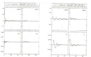
x2 , x3 and λ are showing the peak responses in the region of the lowest frequency 1.795Hz. The variables γ1 , γ2 and γ are showing the peak responses at
2.129Hz, as shown in Figure 5. In the remaining part, all the variables are showing very low responses. This shows that the first two frequencies are the most important ones in the practical point of view. In order to have a comparative study of various variables, the
variations of 𝒙�𝟏 , 𝒙�𝟐 , 𝒙�𝟑 and 𝝀� shown Figures 4(a),
4(b), 4(c) and 4(d) are shown in one Figure 4(e).
k1 = 2×105, k2 = 0.5×105, k3 = 0.5×105 N/m ,
This shows that at resonating frequency, 𝒙�R 1
and 𝒙�R3
are

L1 = 1.0, L2 = 2.5 and B = 0.75 m

The natural frequencies, fn (in Hz) are obtained as,

Group 1	1.795, 3.869, 11.290, 11.446
Group 2	2.129, 18.873, 18.904

All these seven frequencies are to be taken as natural frequencies of the total system. The resonance may occur whenever the exciting frequency matches with any one of these natural frequencies. The values of the natural frequencies are comparable in magnitude with those reported in the literature, which are for some other similar vehicles. The fundamental frequency is found to be 1.795 Hz. It is observed that the highest frequencies in each group are very close to each other. The notable frequencies may be the lowest ones only. The frequency of excitation ( f in Hz) depends on the road roughness. If the road profile is approximated as a sin wave of wave length L and the vehicle is moving with a velocity V, the frequency of excitation may be expressed as
taking almost same values. In the remaining part, 𝒙�R 3 is much less than 𝒙�R 1 . Figure also shows that the displacement undergone by the rear axle 𝒙�R 2 is much
smaller than the displacement undergone by the front
axle 𝒙�R 1 . The figure shows that the disturbance given at the front wheel is also producing pitch motion 𝝀� , but
this is very small in comparison to the other variables.
The variations of 𝜸�R 1 , 𝜸�R 2 and 𝜸� shown in Figures 5(a),
5(b), and 5(c) are shown in one place as in Figure
5(d). It is observed that the value of the roll motion of the main body γ is in between the values of roll motions of the front axle and rear axle. At high frequencies γ is almost negligible.

f = V/L (21)

It is to be observed that the frequency of excitation increases with increase in the velocity or decrease in the wave length.

4. Frequency Response of the System

In order to excite the system with a harmonic forcing function, the excitation is given at one of the front wheels as

International Journal of Scientific & Engineering Research, Volume 4, Issue 9, September-2013 2109

ISSN 2229-5518

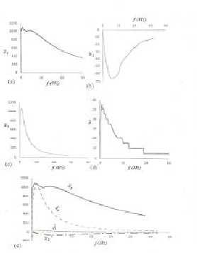
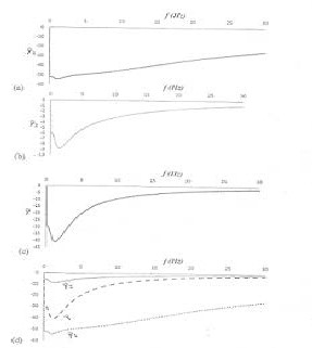
Figure 4 Frequency response

Figure 5 Frequency response

5. Transient Response of the System

The Equations (9a and 9b) are integrated for pulse input given at the wheels. Verities of pulses are tried and the time responses are obtained. Few typical cases are presented here. A pulse input is given to right side front wheel [y1 (0) = 0.1m] and the responses are presented in Figures 6. It is observed that the front axle is undergoing maximum oscillations and rear axle is undergoing very less oscillations; the front axle is also undergoing very small roll motion. The rear axle is undergoing negligible amount of roll motion. The reason may be the disturbance is closer to

front axle. It is also to be observed that the body of the vehicle is undergoing roll and pitch oscillations in addition to up and down vertical motion. It is observed that vertical motion of the main body is very small in comparison to the vertical motion of the front axle. Similarly, roll and pitch motions are small in comparison to the roll motion of the front axle. In order to study the effect of damping on comfort level of the passengers, a quantity z2 which is the sum of the squares of vertical displacements at each corner of the vehicle is evaluated. The variation of z2 with time is also shown.
An impulse disturbance is next given to the right side
front wheel [ 𝒚𝟏 (0) = 500m/s] and the responses
obtained are presented in Figure 7. It is observed that
the rear axle is also under going small oscillations. The body of the vehicle is undergoing oscillations which are more than the previous case. This shows that an impulse disturbance is more severe than a pulse displacement disturbance. It is to be observed that the oscillatory motion of the main body is much less than oscillatory motion of the front axle and, oscillatory motion of the rear axle is much less than the oscillatory motion of the main body. It is also observed that the roll motion of the main body is much less than the roll motion of the front axle and, the roll motion of the rear axle is much less than roll motion of the main body. Further, the roll motion and pitch motion of the main body are almost comparable in magnitude. It is also to be observed that the value of z2obtained with pulse displacement is much higher than that obtained with impulse disturbance. The reason could be, in the later case the main body is undergoing roll and pitch motions, whereas in the in the former case the roll and pitch motions of the main body are very small. On the whole it is noted that when a disturbance occurs, the axles takes the

maximum vibrations leaving very little to main body. The authors tried various combinations of disturbances and studied the responses.

Figure 6 Time response due to pulse displacement disturbance.

International Journal of Scientific & Engineering Research, Volume 4, Issue 9, September-2013 2110

ISSN 2229-5518

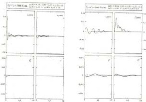
Figure 7 Time response due to impulse displace- ment disturbance.

6. Concluding Remarks

The work present this paper may be summarised as follows.

References

17th International Symposium on mathematical theory of networks and Systems, Japan, July 2006.

5. Wei Gao, Nong Zhang, Dynamic analysis of vehicles with uncertain parameter, 14th International congress on Sound and Vibration, Australia, July

2007.

6. Kamalakannan, K., Elaya Perumal, A., Mangalaramanan, S., Arunachalam, K., Performance analysis of behaviour characteristics of CVD (semi active )in quarter car Model, Jordan Journal of

Mechanical and industrial engineering, Vol. 5, June 2011, pp. 261 – 265.

7. Sawant, S.H., Belwakar,V., Kamble, A., Pushpa, B., and Dipali Patel, D., Vibrational analysis of

quarter car vehicle dynamic system subjected to harmonic excitation by road surface, Undergraduate Academic Research Journal ,Vol.

1, 2012, pp. 46 – 49.

8. Thite, A.N., Devolopment of a refined quarter car model for the analysis of discomfort due to vibration, Advances in Acoustics and Vibration, Hindawi

Publishing Corporation, 2012.

9. Gadhai Ustav, D., Sumanth, P., Quarter model amalysis of Wagon-R Car’s rear suspension using ADAMS, International Journal of Engineering Research and Technology, Vol.1, 2012, pp.1 – 5.

10. Lin, Y., and Kortum, W., Identification of system physical parameters for vehicle systems with nonlinear components, International Journal of Vehicle Mechanics and Mobility, Vol.46, No.12,

2007, pp. 354 – 365.

11. Husenyin Akcay, and Semiha Turkay, Influence of tire on mixed H 2 / H∞ synthesis of half car active suspensions, Journal of Sound and Vibration, Vol.322, 2009, pp.15 – 28.

12. Li-Xing Gao, and Li-Ping-Zing.,Vehicle vibration analysis in changed speeds solved by pseudoexcitation method, Mathematical Problems in Engineering, Hindawi Publishing Corporation,

2010.

13. Thite, A.N., Banvidi, S., Ibicek, T., and Bennett, L., Suspension parameter estimation in the frequency domain using a matrix inversion approach, International Journal of Vehicle

Mechanics and Mobility, Vol.49, No.12, 2011, pp. 1803 – 1822.

14. Roberto Spinola Barbosa, Vehicle vibration response subjected to long wave measured pavement roughness, Journal of Mechanical Engineering and Automation, Vol. 2, No.2, 2012, pp. 17 – 24.

15. Libin Li, and Qiang Li., Vibration analysis based on

International Journal of Scientific & Engineering Research, Volume 4, Issue 9, September-2013 2111

ISSN 2229-5518

Analysis of chaotic vibration of nonlinear seven degree of freedom full car model, 3rd International Conference on Integrity, Reliability and Failure, Portugal, July 2009.

19. Ikbal Eski, and Sahin Yildirim, Vibration control of vehicle active suspension system using a new robust

neural network control system, Journal of

Simulation Modelling Practice and

Theory,Vol.17, 2009, pp.778 – 793.

20. Guidaa, D., Nilvetti,F., and Pappalardo, C.M., Parameter identification of full-car model for active suspension design, Journal of Achievements in Materials and Manufacturing Engineering,

Vol.40, No. 2, 2010, pp.138 – 148.

21. Kasi Kamalakkannan, Elayperumal, A., and Satyaprasad Managalaramam., Simulation aspects of a full-car ATV model semi active suspension, Journal of Scientific Research Engineering,

Vol.4, 2012, pp.384 – 389.