International Journal of Scientific & Engineering Research, Volume 4, Issue 10, October-2013 587

ISSN 2229-5518

Analysis and Simulation of a Single Generator- Infinite Bus Power System under Linear Quadratic Regulator Control

Ayokunle A. Awelewa, Ayoade F. Agbetuyi, Ishioma A. Odigwe, Isaac A. Samuel, Kenechukwu C. Mbanisi

Abstract— The thrust of this article is to develop elaborate educational material on linear quadratic regulator (LQR)-based power system control for electrical engineering students, especially senior undergraduate and fresh graduate students. The paper considers a comprehensive description of a power system, which is represented by a network of a single generator connected to an infinite bus, highlighting modeling, analysis, and simulation of the system. Graphical outputs for various combinations of system state and input weighting matrices are presented.

Index Terms— controllability and observability, linear quadratic regulator, model, single generator-infinite bus power system, state matrix, weighting matrix.

1 INTRODUCTION

——————————  ——————————
ower system networks are interconnections of generat- ing stations and loads by means of transmission lines that span several kilometers. The lines are high-tension
cables that connect the generation to the transmission/sub- transmission substations and distribution cables that ultimate- ly supply the customer loads. Moreover, a typical power sys- tem is a huge, complex network whose constitutive devices have different characteristics and response rates [1]. Therefore, its planning, design, operation, and maintenance require proper analysis and thorough understanding of various ele- ments that compose it. It is, however, desirable that these ele- ments operate together to ensure reliable, secure, and stable performance of the system at all time. Yet negative conditions or disturbances, such as single-phase to ground fault, three- phase to ground fault, sudden outage of large generation or load, etc., which may adversely affect the system do occur. Although the effect of these disturbances vary in degree de- pending on their location, type, and magnitude, their overall consequence is to shift the system from its steady-state opera- tion, thereby making interconnected generators lose synchro- nism. So a significant power system operating criterion is that generating units remain in synchronism [1] during normal and abnormal conditions such that the system is kept stable and secure. Meanwhile, synchronous generator excitation control constitutes one of the most widely used methods to effect res- toration of system stability—especially to dampen out local plant and inter-area mode oscillations—after the system has been perturbed [2], [3] and many excitation control schemes based on optimal control have been developed [4], [5], [6]. But the aim of this work is to use a simplified power system net- work to show the effect of varying system state and input weighting matrices on the dynamic performance of a power system. And this is particularly useful to beginners in the study of power system dynamics and control.
The rest of the paper is organized as follows. In section 2 a detailed description of the power system model employed is
presented. In Section 3 a brief overview of linear quadratic regulator control is covered. Graphical outputs from system simulation as well as discussion of results are outlined in Sec- tion 4, and conclusions are drawn in Section 5.

2 SYSTEM MODEL AND ANALYSIS

The power system network considered in this work is a single synchronous generator connected to an infinite bus. The gen- erator and the infinite bus are interconnected through a num- ber of transmission lines. A generic representation of this is shown in Fig. 1 [7], and a concise description, depicting a re- sultant impedance for all intermediate impedances between the generator and the infinite bus, is given by Fig. 2, where Rr and Xr are the resultant resistance and reactance, respectively.
Fig. 1. Generic representation of an SMIB.

Fig. 2. Concise representation of an SMIB.
The considered network model, which comprises third-order
state-space equations, is derived from the generator electro- mechanical performance equations as well as the equations representing the relationships between generator quantities, transmission line parameters, and infinite bus quantities. For

International Journal of Scientific & Engineering Research Volume 4, Issue 10, September-2013 588

ISSN 2229-5518

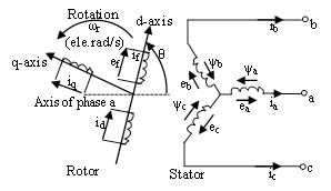
equations capturing the electrical characteristics of the genera- tor, Fig. 3 [7] is apt. Here the dq0 transformation based on the two-reaction theory of synchronous machines [8] is employed. The transformation is a procedure for mapping the three phases of a synchronous generator into equivalent three ax- es—d-axis, q-axis, and zero-axis. (The zero-axis is a fictitious neutral axis included in order to have a valid invertible trans- formation.)
flux linkages
• ψfd , ψ1d , ψ 1q : field and damper circuit flux linkages
• Lad : d-axis mutual or magnetizing inductance
• Laq : q-axis mutual or magnetizing inductance
• Lfd , L1d , L 1q : rotor circuit leakage inductances
• Ll : stator circuit leakage inductance
• L0 : neutral axis inductance
• p : differential operator (d/dt).
Equations (1)-(12), which are all given in per unit, form the
fundamental expressions that completely depict the electrical
characteristics of a synchronous generator. (The derivations
are well spelt out in [7].)
To complete the mathematical equations of a synchronous generator, equations of motion (often called swing equation) showing its mechanical characteristics are given by [11], [12]

dδ dt = ω

(13)
Fig. 3. Stator and rotor circuits of a synchronous

d 2δ

where

dt 2 = 12H (Pm − Pe − D dδdt ) ,

(14)
generator.
In generating the electrical equations, one damper circuit
each is located on the d-and q-axis, and the assumptions of
sinusoidal distribution of stator windings along the air gap, negligibility of magnetic saturation and hysteresis effects, and constant rotor inductances vis-a-vis rotor position are consid- ered [9], [10]. For stator circuits, the equations [7] are
δ = rotor angle (radians)
ω = rotor angular velocity (radians/s)
Pm = mechanical input power in per unit
Pe = electrical power in per unit
H = inertia constant in per unit
D = damping coefficient.
The electrical power in (14) is given in terms of the dq0 quanti-

v d = pψ d − ψ q ω r − R a i d

vq = pψq + ψd ωr − R a i q

v0 = pψ0 − R a i 0

(1) (2)
(3)
ties as [7]

Pe = v d i d + v d i q + 2v 0i 0 .

And for a balanced system, (15) leads to

Pe = v di d + v di q .

(15)
(16)

ψ d = −(L ad + L l )i d + L adi fd + L adi1d

ψ q = −(L aq + L l )i q + L aqi1q

ψ 0 = −L 0i 0

(4) (5)
(6)
For a lossless transmission line, i.e., Re = 0 in Fig. 2, the equation relating the generator currents to the infinite bus bar voltage can be expressed as [9]

v q − Ecosδ

i d =

and for rotor circuits, the equations [7] are

v fd = pψ fd + R fdi fd

0 = pψ1d + R1d i1d

0 = pψ1q + R1q i1q

(7) (8)
(9)

x e

Esinδ − vd

i q = x e ,

where E is the infinite bus bar voltage.
(17)
(18)

ψ fd = (L fd + L ad )i fd + L adi1d − L adi d

ψ1d = L adi fd + (L1d + L ad )i1d − L adi d

ψ1q = (L1q + L aq )i1q − L aqi q ,

(10) (11) (12)

Furthermore, neglecting the damper circuits, armature re-
sistance, and the transformer voltage terms, pψd and pψq , while assuming constant rotor speed [13], the combined volt-
age and flux linkage equations are
where
• vd ,vq ,v0 : d-axis, q-axis, and neutral axis respective voltages
• vfd : field voltage

v d

v q

v fd

and

= −ω0ψ q

= ω0ψ d

= pψ fd + R fdi fd

(19)
(20) (21)
• id ,iq ,i0 : d-axis, q-axis, and neutral axis respective currents

ω0ψ d = −(X ad + X l ) i d + X adi fd

(22)
• ifd ,i1d ,i1q : field and damper circuit currents
• Ra : armature resistance per phase
• Rfd ,R1d ,R1q : rotor circuit resistances

ω0ψ q

ω0ψ fd

= −(X aq + X l )i q

= −X adi d + (X ad + X fd ) i fd ,

(23)
(24)
• ψd , ψ q , ψ0 : d-axis, q-axis, and neutral axis respective
respectively.

International Journal of Scientific & Engineering Research Volume 4, Issue 10, September-2013 589

ISSN 2229-5518

2.1 Nonlinear State-Space Model

Equations (13)-(24) are now used to develop the state-space equations. The swing equations, (13) and (14), constitute the

∆Ω

where

= A∆Ω + B∆u

(30)
first two state equations in which the rotor angle and the

 ∆δ 

speed deviation are the state variables, i.e.,

∆Ω = 

∆ω 

δ = ω

(25)

∆ψ f 

ω = 1M (Pm − Dω − Pe ).

(26)
The equation describing Pe in terms of the network variables and parameters is derived in Appendix I (see (A.12)–(A.14)).
The third state variable is normally chosen to account for the field circuit dynamics, and therefore, the choice of field flux linkage, ψfd , is most appropriate. In some literature [14], [15], E΄q , which is the q-axis component of the voltage behind transient reactance Χ΄d , is chosen as the third state variable, but this choice is equivalent to that of the field flux linkage because the two variables are related by

 ∂f1

 ∂δ

 ∂

A = 

 ∂δ

 ∂f3

 ∂δ

 

∂f1

∂ω

∂f 2

∂ω

∂f3

∂ω

∂f1 

∂ψ f 

∂f 2 

∂ψ f 

∂f3 

∂ψ f 

E ' =

Lad ψ

 0 

=  

q Lffd fd

(27)

B 0

 ∂f3 

The third equation is now given by (28). (See (A.1)–(A.11) in  
Appendix I.)

 ' 

and

 ∂u 

(X d + X e )ψ f

 X d − X d Ecos δ

f (Ω , u

) = δ

pψ f

= u −



+ 



+ X e do



 

d + X e 

1 0 0 ,u

f Ω , u = ω

( )

  

 (28)

2 0 0

 ,u

The complete non-linear state-space model [2], [16], [17] of
the system is given by (29) below.

f3 (Ω0

, u 0

) = ψ f ,u

δ = ω

ω = B1 − A1ω − A 2ψ f sinδ − 2 sin2δ

(29)

∆δ = δ − δ0 ≡ ∆δ = δ − f1(Ω 0 , u 0 )

∆ω = ω − ω0 ≡ ∆ω = ω − f 2 (Ω 0 , u 0 )

ψ f

= u − C1ψ f

+ C 2cosδ

∆ψ f

= ψ f

− ψ f 0 ≡ ∆ψ f

= ψ f

− f 3 (Ω 0 , u 0 )

where

A1 = D ; A 2 = E ;

∆u = u − u 0 .

M M X ' + X

T '

2.3 System Stability and State Matrix Analysis

 d e  do

 

The parameters of the system considered in this work are [2]:

E 2  X '

− X q 

Xd = 1.25
X' = 0.3
Xq = 0.7
T' = 9.0

 d 

B1 = ; B 2 = ;

M = 0.0185
D = 0.005
Xe = 0.2
E = 1.0

M M X '

+ X e (X q + X e )

The initial values of u and Pm are assumed to be 1.1p.u. and

 d 

 

0.725p.u. respectively, while the steady-state values of the sys- tem variables are given as [2]:

 − ' 

δi = 0.7438

ωi = 0

ψ fi = 7.7438

(X d + X e )

 X d

X d E

From the above-given information, the values of A , A , B ,

C1 =

; C 2 =   .

1 2 1

 X ' + X

T '

 X '

+ X e 

B2 , C1 , C2, are computed as A1 =0.270, A2 = 12.012, B1 = 39.189,

 d e  do

 

 d 

 

B2 = -48.048, C1 = 0.323, and C2 = 1.9, and are used to evaluate all the elements of the Jacobian (state) matrix, A, and those of

2.2 Linearized System State-Space Model

the input vector, B, in the linearized system model as follows:
The aforementioned model can further be simplified by linear- izing it about a known operating point. This is carried out by using the Taylor series expansion technique.
Therefore, expanding the non-linear state equation of eqn. 29 into a Taylor series about Ω0 = [δ0 ω0 ψf0 ] and neglecting all the higher-order terms yields the matrix-form representation given by

∂f1

∂δ

Ω ,u

= 0;

∂f1

∂ω Ω ,u

= 1;

∂f1

∂ψ f

= 0

Ω ,u

International Journal of Scientific & Engineering Research Volume 4, Issue 10, September-2013 590

ISSN 2229-5518

∂f 2

∂δ

∂f 2

Ω ,u

= 48.048 cos 2δ0 − 12.012ψ f 0 cos δ0

= −64.534;

= −0.270;

3 LQR DESIGN

The linear quadratic regulator establishes an optimal control law for a linear system with a quadratic performance index. Given the linearized system model in (31), the problem here is to determine the matrix K of the optimal control law

∂ω

∂f 2

Ω ,u

= −12.012 sin δ0 = −8.1533;

∆u = −KΔΩ
in order to minimize the performance index

∞

(34)

∂ψ f

Ω ,u

J =  ΔΩ T



QΔΩ + ∆u T

R∆u dt,



(35)

∂f 3

∂δ

Ω ,u

∂f 3

= −1.9 sin δ0 = −1.2896; ∂ω

Ω ,u

= 0;

where Q is a positive-definite (or positive-semidefinite) Her- mitian or real symmetric matrix, R is a positive-definite Her-

∂f 3

= −0.323;

∂f 3

= 1.

mitian or real symmetric matrix, and ΔΩ is the state vector.

0 0 0 0

And substituting these values into (30) leads to (31) below.

∞

T  T 

 ∆δ   0

1 0 

∆δ 

 0 

J = ∫ ∆Ω

 Q + K

RK ∆Ωdt

(36)

  

    0  

 ∆ω

 =  − 64.534

− 0.270

− 8.1533

∆ω  +  0 ∆u

 ∆ψ f 

 − 1.2896 0

− 0.323  ∆ψ f 

 1 

Thus minimizing J in (36) results in the gain matrix [18], [19]

  

 

 

(31)

K = R

−1B T P,

(37)
The stability of the linearized system can now be deter- mined using the Lyapunov’s indirect stability method (other-
where P is a positive-definite Hermitian or real symmetric
matrix that satisfies the reduced Riccati equation
wise known as the second method of Lyapunov). It states that if a non-linear system is linearized about its operating point, and it’s observed that the resulting linearized model is strictly stable (i.e., all the eigenvalues of its state matrix are strictly in the left-half complex plane), then the equilibrium point for the

A T P + PA − PBR −1B T P + Q = 0,

4 SYSTEM SIMULATION

(38)
actual non-linear system is asymptotically stable [15]. Compu- ting the eigenvalues, λ1 , λ2 , λ3 , of the system using the MATLAB function eig, we have λ1 = -0.2165 + 8.0315i, λ2 = -
0.2165 – 8.0315i, and λ3 = -0.16, so the stability condition is met. Likewise, the state controllability and observability of the system can be determined by performing the Kalman test [18]. It states that a dynamical system is completely state controlla-
ble if and only the rank of an n x n controllability matrix
The system is now simulated in MATLAB to show its perfor-
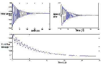
mance for various sets of values of Q and R. First, the open-
loop behavior of the system is shown in Fig. 4. Then for the
closed-loop (LQR-controlled) system performance, two cases
of the weighting matrices Q and R are considered. In the first
case, R is fixed and Q is varied, while in the second case R is
varied and Q is fixed.
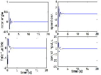
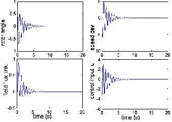
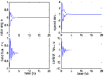
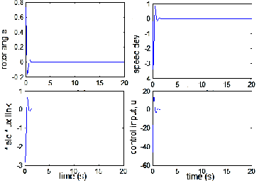
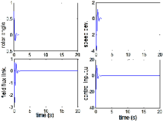
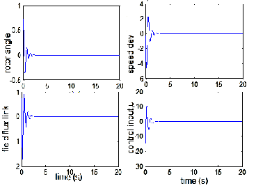
So the responses in Figures 5-8 show the case when R = 1 and

[B AB

A 2B 

A n −1B]

(32)

Q = 0.1*I, I, 5*I, and 15*I, and likewise, those in Figures 9-11 show the case when Q = 15*I and R = 0.1, 0.2, and 0.8. (Here I

is n; also, the system is completely state observable if and only if the rank of an n x nm observability matrix
is 3 x 3 identity matrix.)

 C 

 CA 

 CA 2 

  

CA

n −1 



(33)
is n. (Here n represents the order of the system and m the number of system outputs.)
Therefore, using (32) and (33), we can find the controllability and observability matrices (indicated by M and N, respective- ly) of the system given in (31) as

 0 0



− 8.1533



 1 0



− 64.5340 



M =  0

− 8.1533

4.8349 ; N =  0 1

− 0.2700 .

 − 0.3230

8.1043 

 − 8.1533 

Fig. 4. System open-loop characteristics.

International Journal of Scientific & Engineering Research Volume 4, Issue 10, September-2013 591

ISSN 2229-5518

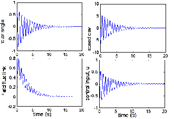
Fig. 5. LQR-controlled system characteritics (when Q = 0.1*I;

R = 1).
Fig. 6. LQR-controlled system characteritics (when Q = I;

R = 1).
Fig. 7. LQR-controlled system characteritics (when Q = 5*I;
R = 1).
Fig. 8. LQR-controlled system characteritics (when Q = 15*I;

R = 1).
Fig. 9. LQR-controlled system characteritics (when Q = 15*I;

R = 0.1).
Fig. 10. LQR-controlled system characteritics (when Q = 15*I;
R = 0.2).

International Journal of Scientific & Engineering Research Volume 4, Issue 10, September-2013 592

ISSN 2229-5518

Substituting (A1) into (22) gives

0 d ad l d

ad vfd + Ladidp 

ω ψ = −(X

+ X )i + X

 (Lad

+ Lfd

)p + R



fd 

= Xadvfd



−  Xad + Xl −

XadLadp 

(Lad

+ Lfd )p +

R fd



 ( ) (Lad

 +

+ Lfd )p +



R fd  d



 Xad Lfdp +  Ladp

Lfd fd

p Xl  + Xad

+ Xl 

= vfd

Xad − 

R  R  

1 + Td' op

Rfd 





 

 d

1 + Td' op 



 

 1 

LadLf

+ (Lad + Lfd )Ll p + 1 

= vfd

Xad −  Rfd  Lad + Ll

Lad + Ll 

X i

1 + Td' op

Rfd 





1 + Td' op

 d d





u + pTd' o Xd − X'd id

Fig. 11. LQR-controlled system characteritics (when Q = 15*I; =

 



 − Xdid ≡ Xadifd − Xdid

(A2)
R = 0.8).
From the analysis of the system characteristics, it could be inferred that though the system is stable, controllable and ob- servable, oscillations of the system variables (rotor angle, for instance) take unbearably and undesirably long time (more than 25s) to dampen out. Also, it could be inferred that the

1 + Tdop

Variable u in (A2) is defined as

u = vfdXad .

Rfd

Let Em (where Em is an arbitrary variable) be given as
performance of the system, when controlled by the LQR, var-  
ies depending on the combination of the state and control weighting matrices, Q and R. When R is fixed and Q is gradu- ally increased, the system dynamic performance shows signif-

Em = Xadifd =

u + pTd' o Xd − X'do id

 

1 + Td' op

(A3)
icant improvement with a price of increased control effort
though. Specifically, better performance is recorded when Q =
15I and R =1 than at any other value of Q with the same R. It
is also observed that with this value of Q and varying values
of R, the behavior of the system improves greatly appreciably.
Notably, at Q = 15I and R= 0.1, best dynamic performance is
Also, from (21), a new term pψf is obtained in terms of pψfd
as illustrated below.

pψfd = vfd − R fdifd = R fd (u − Xadifd )

Xad

Hence,
realized without much control activity—the maximum over- shoot and the settling time for rotor angle are 0.033 and 1.5s,

pψf = u − Xadifd = u − Em,

where
(A4)
respectively.

ψf =

Xad ψfd. R fd

5 CONCLUSION

And by combining (A3) and (A4), ψf can be expressed as

 

A description, analysis, and LQR-based control of a single

ψf = Td' o Em −  Xd − X'd  id 

(A5)
generator connected to an infinite bus have been considered in this paper. Specifically, stability, controllability, and observa- bility of the system have been established using a linearized version of the nonlinear model describing the system. Also,

   

 

Again, from (19), (20), (23), and (A2), vd and vq can be ob- tained as
investigation of the system dynamic performance has been carried out under linear quadratic regulator control for vari- ous combinations of input and state weighting matrices, with

vd = Xqiq

vq = Em − Xdid

(A6)
(A7)
well displayed graphical outputs to show the results of the
By using (A6) and (A7), (17) and (18) can be rewritten as
system simulation.

id = Em − Ecosδ

Xd + Xe

(A8)

APPENDIX

iq = Esinδ

Choosing ψfd as the third state variable, we can derive (28) in

Xq + Xe

(A9)
the body of the paper as follows:
Combining (21) and (24) and solving for ifd result in
Em can now be obtained in terms of ψf by using (A5) and
(A8).

ifd =

vfd +Ladidp

(Lad + Lfd )p + Rfd .

(A1)

International Journal of Scientific & Engineering Research Volume 4, Issue 10, September-2013 593

ISSN 2229-5518

Em =

(Xd + Xe )ψf



 Xd





− X Ecosδ



(A10)

2002.

[12] P.M. Anderson and A.A. Fouad, ‘’Power System Control and Stability,’’ The

IEEE Press, Power Engineering Society, Piscataway, NJ, 2003.

[13] M.S. Ghazizadeh and F.M. Hughes, ‘‘A generator transfer function regulator

 X'd + Xe Td' o

 X'd + Xe 

for improved excitation control,’’ IEEE Transactions on Power Systems, vol.

   



 

By using (A10), (A4) can be rewritten as

13, no. 2, pp. 435-441, May 1998.

[14] D. Gan, Z. Qu and H. Cai, ‘‘Multi-machine power system excitation control design via theories of feedback linearization control and robust control,’’ In-

pψ f

= u −

(X d + X e )ψ f



 X d

+ 



− X Ecosδ



(A11)

ternational Journal of Systems Science, vol. 31, no. 4, pp. 519-527, 2000.

[15] Jean Jaques E. Slotine, and Weiping Li, ‘’Applied Non-linear Control,’’ Pren- tice-Hall Edition, New Jersey, 1991.

 X 'd + X e Td' o

 X 'd + X e 

[16] P.C. Park, ‘‘Lyapunov redesign of model reference adaptive control systems,’’

   

 

  

Equation (A11) is now the third state equation (see (28)).
Also, an expression for Pe is computed by using (16) and (A6)
– (A10) as follows

IEEE Transactions, Automatic Control, AC-11, pp. 362-365, 1989.

[17] M. Nambu and Ohsawa Y., ‘‘Development of an advanced power system stabilizer using a strict linearization approach,’’ IEEE Transactions on Power Systems, vol. 11, pp. 813-818, 1996.

[18] K. Ogata, “Modern Control Engineering,” Third Edition, Prentice Hall, Upper

Pe = vdid + vqiq = Xqiqid + Emiq − Xdidiq

Also,
(A12)

Saddle River, New Jersey, 1997.

[19] R.S. Burns, ‘‘Advanced Control Engineering,’’ Butterworth-Heinemann Edi- tion, Woburn, 2001.

(Xq − Xd )Esinδ

Esinδ

(Xq − Xd )E2sin2δ

Pe = (Xq + Xe )(Xd + Xe ) Em + Xq + Xe Em − 2(Xq + Xe )(Xd + Xe ),

which, after simplification, gives

 X 'd − X q E 2sin2δ

Ayokunle A. AWELEWA is with the Department of Electrical & Infor-

mation Engineering, Covenant University, Canaan Land, Ota, Nigeria. His research areas include power system stabilization and control, and

modeling and simulation of dynamical systems.

 

Pe =



Eψ f sinδ



+  

(A13)

Ayoade A. Agbetuyi is with the Department of Electrical & Information

Engineering, Covenant University, Canaan Land, Ota, Nigeria. His re-

 X 'd + X e Td' o

2(X 'd + X e )(X q + X e )

search areas include renewable energy, power system stability and relia-



 bility, and distributed generation and renewable energy.

REFERENCES

[1] CIGRE Joint Task Force on Stability Terms and Definitions, “Defini- tion and Classification of Power System Stability,” IEEE Trans. Pow- er Systems, vol. 19, no. 2, pp. 1387-1401, May 2004.

[2] L.N. Wedman and Y.N. Yu, ‘‘Computation techniques for the stabili-

zation and optimization of high order power systems,’’ IEEE Power

Industry Computer Applications Conference Record, pp. 324-343,

1969.

[3] P. Kundur, D.C. Lee and H.M. Zein El-Din, ‘‘Power system stabi-

lizers for thermal units: Analytical Techniques and on-site valida-

tion,’’ IEEE Transactions, Vol. PAS-100, pp. 81-95, January 1981.

[4] Q. Lu and Z. Xu, ‘‘Decentralized non-linear optimal excitation con-

trol,’’ IEEE Transactions on Power Systems, vol. 11, no. 4, pp. 1957-

1962, November 1996.

[5] S. Takada, ‘‘Compensation of bus voltage fluctuation by means of optimal control of synchronous machine excitation,’’ Elec. Eng. Jap. (USA), vol. 8, pp. 42-52, 1968.

[6] A. Ghandakly, P. Kronegger, “An Adaptive Time-Optimal Controller for Generating Units Stabilizer Loops,” IEEE-PES Trans. Power Sys- tems, vol. PWRS-2, no. 4, pp. 1085-1090, November 1987.

[7] P. Kundur, ‘‘Power system analysis and control,’’ McGraw-Hill Book

Company, New York, 1994.

[8] G. Krong, ‘‘Two–reaction theory of synchronous machines-part 2,’’ AIEE Transactions, vol. 52, pp. 352-355, June 1933.

[9] B.K. Mukhopadhyay and M.F. Malik, ‘‘Optimal control of synchronous ma- chine excitation by quasilinearisation techniques,’’ IEEE Proceedings, vol. 119, no. 1, pp. 91-98, 1972.

[10] M.F. Hasan and M.G. Singh, ‘‘A hierarchical model-following controller for certain non-linear systems,’’ Int. J. Systems Sc., vol. 7, no. 7, pp. 727-730, 1976.

[11] H. Saadat, ‘‘Power System Analysis,‘‘ McGraw-Hill Book Company, Tata,

Ishioma A. Odigwe is with the Department of Electrical & Information Engineering, Covenant University, Canaan Land, Ota, Nigeria. His re- search areas include distribted generation with renewable energy sources, and power system stability analysis.

Isaac A. SAMUEL is with the Department of Electrical & Information Engineering, Covenant University, Canaan Land, Ota, Nigeria. His re- search areas include power system operation, reliability, and maintenance.

Kenechukwu C. Mbanisi is a former student (September 2008- July 2013) of the Department of Electrical & Information Engineering, Covenant University, Ota, Nigeria. He is profoundly interested in and enthusiastic about modeling, analysis, and control of dynamical systems.

Internatio nal Jo urnal of Scientific & Engineering Research Volume 4, Issue 10, September-2013

ISSN 222S-5518

594

IJSER lb)2013

http ://www.ij se rorq