International Journal of Scientific & Engineering Research, Volume 2, Issue 12, December-2011 1

ISSN 2229-5518

An Efficient Algorithm for Segmentation Using Fuzzy Local Information C-Means Clustering Sandeep Kumar Mekapothula*

Department of ECE, RISE Groups, Ongole, Andhra Pradesh, India

V. Jai Kumar2

Department of ECE, QISCET, Ongole, Andhra Pradesh, India

ABSTRACT - In this paper there is a variation of fuzzy c-means (FCM) algorithm is presented that provides image clustering. The proposed algorithm incorporates local spatial information and gray level information in a novel fuzzy way. The new algorithm is called fuzzy local information C-Means (FLICM). By using this algorithm we can overcome the disadvantages of the previous algorithms and at the same time enhances the clustering performance. The major characteristic of this FLICM is the use of a fuzzy local (both spatial and gray level) similarity measure, aiming to guarantee noise insensitiveness and image detail preservation. Furthermore, the proposed algorithm is fully free of the empirically adjusted parameters (a, λg, λs, etc.). Experiments performed on some synthetic and real images shows that this algorithm is effective and efficient, providing high robustness to noisy images.

Index Terms- Clustering, Fuzzy C-means, Fuzzy constraints, gray level constraints, image segmentation, and spatial constraints.

——————————  ——————————

I. INTRODUCTION

mage Segmentation is one of the first and most important tasks in image analysis and computer vision.

In the literature, various methods have been proposed for object segmentation and feature extraction, described in references. However, the design of robust and efficient segmentation algorithms is still a very challenging research topic, due to the variety and complexity of images. Image segmentation is defined as the partitioning of an image into non-overlapped, consistent regions which are homogeneous in respect to some characteristics such as intensity, color, tone, texture, etc. The image segmentation can be divided into four categories: thresholding, clustering, edge detection and region extraction. In this paper, a clustering method for image segmentation will be considered.
Clustering is a process for classifying objects or patterns in such a way that samples of the same cluster are more similar to one another than samples belonging to different clusters. There are two main clustering strategies: the hard clustering scheme and the fuzzy clustering scheme. The conventional hard clustering methods classify each point of the data set just to one cluster. As a consequence, the results are often very crisp, i.e., in image clustering each pixel of the image belongs just to one cluster. However, in many real situations, issues such as limited spatial resolution, poor contrast, overlapping intensities, noise and intensity in homogeneities reduce the effectiveness of hard (crisp) clustering methods.
Fuzzy set theory [3] has introduced the idea of partial membership, described by a membership function. Fuzzy clustering, as a soft segmentation method, has been widely studied and successfully applied in image clustering and segmentation [4]-[9]. Among the fuzzy clustering
methods, fuzzy c-means (FCM) algorithm is the most popular method used in image segmentation because it has robust characteristics for ambiguity and can retain much more information than hard segmentation methods [11]. Although the conventional FCM algorithm works well on most noise-free images, it is very sensitive to noise and other imaging artifacts, since it does not consider any information about spatial context.
To compensate this drawback of FCM, a
preprocessing image smoothing step has been proposed.
However, by using smoothing filters important image details can be lost, especially boundaries or edges. Moreover, there is no way to control the trade-off between smoothing and clustering. Thus, many researchers have incorporated local spatial information into the original FCM algorithm to improve the performance of image segmentation [5], [11], [14].

Fuzzy Local Information C-Means (FLICM) Clustering

Algorithm

Motivated by individual strengths of FCM_S1, FCM_S2, EnFCM, and FGFCM and its variations, we propose, in this paper, a novel and robust FCM framework for image clustering called Fuzzy Local Information C-means (FLICM) clustering algorithm.

A. Introducing the Fuzzy Factor

All the methods described in the previous Section have yielded effective clustering results for images [12], [13], and [16], but still have some disadvantages.
1) Although the introduction of local spatial information enhances their insensitiveness to noise to some extent, they still lack enough robustness [18]-[20] to noise and outliers, especially in absence of prior knowledge of the noise.

International Journal of Scientific & Engineering Research, Volume 2, Issue 12, December-2011 2

ISSN 2229-5518

2) There is a crucial parameter a (or) in their objective functions, used to balance between robustness to noise and effectiveness of preserving the details of the image. Generally, its selection has to be made by experience or trial and error experiments.
3) They are all applied on a static image, which has to be
computed in advance. Details of the original image could
be lost depending on the method used to generate the new image.
In order to overcome the above mentioned disadvantages a
new factor in FCM objective function is needed. The new factor should have some special characteristics:
• To incorporate local spatial and local gray level information in a fuzzy way in order to preserve robustness and noise insensitiveness;
• To control the influence of the neighborhood pixels
depending on their distance from the central pixel.
• To use the original image avoiding preprocessing steps
that could cause detail missing.
• To be free of any parameter selection.
So, we introduce the novel fuzzy factor Gki defined as

(1)

Where, the ith pixel is the center of the local window (for
example, 3x 3), K is the reference cluster and the i th pixel belongs in the set of the neighbors falling into a window around the ith pixel. (Ni). di,j is the spatial Euclidean distance between pixels i and j ,ukj is the degree of membership of the jth pixel in the kth cluster, m is the weighting exponent on each fuzzy membership, uk and is the prototype of the center of cluster .It is easy to see that the factor Gki is completely free of using any parameter that controls the balance between the image noise and the image details. The control of this balance is automatically achieved by the definition of the fuzziness of each image pixel (both spatial and gray level). Also, by using, dij the factor Gki makes the influence of the pixels within the local window, to change flexibly according to their distance from the central pixel. Thus, more local spatial information can be used. It is worth indicating that the shape of the local window used in our experiments is square, but also, windows with other shapes such as diamond or circle can easily be adapted to the algorithm. As a whole, Gki reflects the damping extent of the neighbors with the spatial distances from the central pixel. In contrast, the parameter a(or λ) in FCM_S, EnFCM, FGFCM, and their variants, is globally taken as a constant and, thus, it is relatively difficult to vary adaptively with different spatial locations or distances from the central pixel. Moreover, there is no need of preprocessing steps to apply the algorithm, as it will be shown in the following. The important role of Gki during the application of the algorithm will also be shown in the following subsection.

B. General Framework of FLICM

By using the definition of Gki, we now propose a robust FCM framework for image clustering, named Fuzzy Local Information C-Means (FLICM) clustering algorithm. It incorporates local spatial uki and vk gray level information into its objective function, defined in terms of (2)
The two necessary conditions for Jm to be at its local minimal extreme, with respect to ukj and vk are obtained as
follows: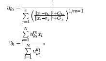
(3,4)
Thus, the FLICM algorithm is given as follows.
Step 1. Set the number C of the cluster prototypes, fuzzification parameter m and the stopping condition.
Step 2. Initialize randomly the fuzzy partition matrix.
Step 3. Set the loop counter b = 0
Step 4. Calculate the cluster prototypes using (4).
Step 5. Compute membership values using (3).
Step 6. If max {U (b) - U (b+1)} < ξ, Then stop, otherwise, set b =

b+1 and go to step 4.

When the algorithm has converged, a defuzzification process takes place in order to convert the fuzzy partition matrix U to a crisp partition. The maximum membership procedure is the most important method that has been developed to defuzzify the partition matrix. This procedure assigns the pixel to the class C with the highest membership.
(4)
It is used to convert the fuzzy image achieved by the
proposed algorithm to the crisp segmented image. The measure used in the FLICM objective function is still the Euclidean metric as in FCM, which is computationally simple. Moreover, differently from FCM, FLICM is robust because of the introduction of the factor Gki which can be analyzed as follows.
The noise tolerance and outliers resistance property, completely relies on the definition of Gki as it is
seen is automatically determined rather than artificially set, even in the absence of any prior noise knowledge. Two basic cases which describe the performance of the algorithm when outliers are present in the window will be presented in the following. As it will be shown the Gki of the noise-corrupted pixels within a window will be kept to similar value to the central pixel ignoring the inﬂuence of the noise. The Gki value will adaptively change in every

International Journal of Scientific & Engineering Research, Volume 2, Issue 12, December-2011 3

ISSN 2229-5518

iteration, converging to the central pixel’s value and thus
preserving the insensitiveness to noise and outliers.
• Case 1: The central pixel is not a noise and some pixels within its local window may be corrupted by noise. An example illustrated in Fig. 1 depicts this situation, in which a 3 X 3 window was used. This window was extracted from the noisy image (marked with a rectangle) shown on the left of the top row of the Fig. 1. It is clearly shown that after ﬁve iterations the algorithm converges and the cor- responding membership values of the noisy, as well as of the no-noisy pixels converge to a similar value, ignoring the noisy pixels Fig. 1(a)–1(d)]. The neighboring pixels, where their corresponding windows are intercovered, are examined as well. Generally, in such cases, the gray level values of the noisy pixels are far different from the other pixels within the window, and thus the factor Gki balances their membership values. Therefore, the combination of the spatial and the gray level constraints incorporated in the Gki suppress the inﬂuence of the noisy pixels, and, hence, the algorithm becomes more robust to outliers.
• Case 2: The central pixel is corrupted by noise, while the other pixels within its local window are homogenous, not corrupted by noise. Such an example is clearly demonstrated in Fig. 2. Again a 3 X 3 window was used, which was extracted from the noisy image (marked with a rectangle) shown on the left of the top row of the Fig.
2. It is shown that after ﬁve iterations the membership value of the noisy (central) pixel converges to a similar to neighboring pixels membership value, ignoring in this way the potential inﬂuence by noise, as shown in Fig. 2(d). Generally, in such cases the factor Gki balances the membership value of the central pixel taking into account the spatial, as well as the gray level of the no-noisy neighboring pixels in a fuzzy manner. Thus, the proposed method becomes more robust to outliers, since the membership value of the central pixel is not inﬂuenced by noise. The above two examples just give some intuitive illustrations about the robustness of our algorithm. The enhancement of its robustness to noise and outliers is based on the incorporation of the Gki with fuzzy spatial and gray level localities constraints (18).
Another issue that is worth to point out is the
denoising potential of the proposed method in comparison
to other methods. FCM_S1 uses a mean-type filtering, so it is relatively suitable for noisy images corrupted by Gaussian noise, whilst FCM_S2 uses a median-type filtering, and as a consequence, it is relatively suitable for images corrupted by impulsive noise. Also, in both cases, the final effectiveness of ignoring the noise in clustering relies on the value of the parameter. Thus, it is generally hard to choose the proper method (FCM_S1 or FCM_S2) and the optimal parameter for good clustering results. On the other hand, FGFCM is independent of the noise type, but its clustering results depend also on parameter.
Parameter has a relatively small value range, and one can reach more easily than FCM_S1 and FCM_S2 the correct parameter. But its selection still needs experience or usage of the trial-and-error method. Compared with FCM_S1, FCM_S2 or FGFCM, FLICM is independent of the type of the noise and completely free of any parameter selection or use. Its denoising performance is shown in the experimental results section.
The factor Gki also seems to preserve more image information. It incorporates both local spatial and gray
level relationship the local spatial relationship changes adaptively according to spatial distances from the central pixel. The local gray level relationship not only varies automatically according to different gray level difference between the pixels over an image, but also is dependent on their fuzzy membership values. Thus, the value of Gki varies from pixel to pixel, as well as from iteration to iteration within a neighborhood window, which likely preserves more information than using the same values for each pixel and iteration. Therefore, FLICM adopting Gki seems able to preserve more image details than the other methods. The major characteristics of the FLICM are summarized below:
• It provides noise-immunity.
• It preserves image details.
• It is free of any parameter selection.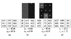

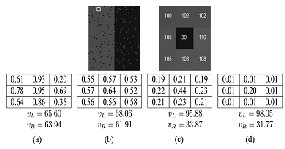
Fig. 1. 3 X 3 window with noise (marked with a rectangle in the initial image), their corresponding membership values and the cluster centers (vL and vR). (a) The initial membership values, (b) after one iteration, (c) after three iterations, (d) after five iterations.
Fig. 2. 3 X 3 window with noise (marked with a rectangle in the initial image), their corresponding membership values and the cluster centers (vL and vR). (a) The initial membership values, (b) after one iteration, (c) after three iterations, (d) after five iterations.

International Journal of Scientific & Engineering Research, Volume 2, Issue 12, December-2011 4

ISSN 2229-5518

IV. EXPERIMENTAL RESULTS

In this section, we show the performance of the proposed method by presenting numerical results and examples on various synthetic and real images, with different types of noise and characteristics. Furthermore, we compare the efficiency and the robustness of FLICM with six fuzzy algorithms FCM_S1, FCM_S2, EnFCM, FGFCM_S1, FGFCM_S2, FGFCM, and two well-known non fuzzy algorithms, k-means [21] and hierarchical clustering based on the SLINK algorithm [22]. The denoising performances of the above nine algorithms were compared with respect to the optimal segmentation accuracy (SA), where SA is deﬁned as the sum of the correctly classiﬁed pixels divided by the sum of the total number of pixels [9] 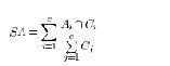(5)
Where c is the number of clusters represents the set of
pixels belonging to the ith class found by the algorithm,
while Ci represents the set of pixels belonging to the ith class in the reference segmented image.
In our numerical experiments, we generally choose
the parameters to be λs =3, ε =0.00001 and NR= 8 (a 3 X 3 window centered on each pixel, except the central pixel itself) [16]. First, we apply these algorithms to a synthetic test image (Fig. 3(a): 128 X 128 pixels, two classes with two gray level values taken as 20 and 120) corrupted by different levels of Gaussian, Uniform and Salt & Pepper noise, respectively. The number of clusters is set equal to c
=2. Also, parameter λg is set equal to λg = 6.0 for FGFCM
and its variants (obtained by searching the interval of [0.5,
6] with respect to SA). The parameter a is chosen equal to a
= 4.2 in all the algorithms FCM_S1, FCM_S2 and EnFCM [12], which is obtained by seeking the interval [0.2, 8]. Fig. 3 illustrates the clustering results of a corrupted by gaussian noise (20%) image. FGFCM_S1 [Fig. 3(f)], FGFCM_S2 [Fig.
3(g)], FGFCM [Fig. 3(h)], k-means [Fig. 3(i)], and SLINK
[Fig. 3(k)] are respectively affected by the noise to different
extents, which indicates that these algorithms lack enough robustness to the gaussian noise. Visually, FCM_S1 [Fig.
3(c)], FCM_S2 [Fig. 3(d)], and EnFCM [Fig. 3(e)] remove most of the noise, but still their results are not satisfactory enough. On the other hand, FLICM [Fig. 3(k)] removes
almost all the added noise achieving satisfactory results, fact that is veriﬁed by the segmentation accuracy (SA) results shown in Table I.
Table I gives the average segmentation accuracy
results of the nine algorithms on the speciﬁc synthetic image corrupted respectively by different noises with different levels. Each experiment has been performed using ﬁve different random initializations and the typical one has been assumed as the result. performance than FCM_S type, EnFCM, FGFCMs, and non fuzzy algorithms, presenting robustness to all considered kind of noises against to the other eight algorithms.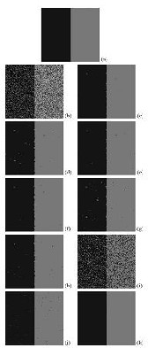

Fig. 3. Clustering of a synthetic image. (a) Original image, (b) the same image with gaussian noise (20%), (c) FCM_S1 result, (d) FCM_S2 result, (e) EnFCM result, (f) FGFCM_S1 result, (g) FGFCM_S2 result, (h) FGFCM result, (i) k-means result, (j) SLINK result, and (k) FLICM result.

TABLE I

Segmentation Accuracy (SA %) of nine algorithms on synthetic images.

	Gaussian	Uniform	Salt & Pepper
	8 %	10 %	15 %	8 %	10 %	15 %	8 %	10 %	15 %
FCM_S1	99.28	98.34	97.21	99.98	99.49	96.54	99.60	99.45	99.10
FCM_S2	99.71	99.34	98.04	99.98	99.76	95.67	99.62	99.53	99.46
EnFCM	99.30	98.36	97.25	99.99	99.52	96.26	99.60	99.45	99.10

International Journal of Scientific & Engineering Research, Volume 2, Issue 12, December-2011 5

ISSN 2229-5518

FGFCM_S1	97.58	97.51	97.04	97.65	97.61	96.41	97.66	97.51	97.34
FGFCM_S2	99.81	99.43	97.72	99.92	99.78	94.25	74.90	74.89	74.88
FGFCM	98.62	98.48	97.60	98.68	98.56	95.92	88.12	86.69	83.33
k-means	92.08	88.96	79.93	82.88	81.55	80.01	92.82	92.78	91.31
SLINK	99.77	99.22	98.49	81.92	68.05	57.92	99.29	99.17	98.68
FLICM	99.89	99.64	98.95	99.98	99.89	98.74	99.9.3	99.91	99.90
	FLICM	87.94	95.18	83.58

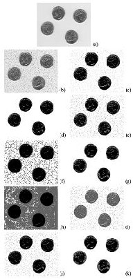
Fig. 4. Clustering of a synthetic image. (a) Original image, (b) the same image with gaussian noise (30%), (c) FCM_S1 result, (d) FCM_S2 result, (e) EnFCM result, (f) FGFCM_S1 result, (g) FGFCM_S2 result, (h) FGFCM result, (i) k-means result, (j) SLINK result, and (k) FLICM result.

TABLE II

Comparison Scores (R %) of nine algorithms on various images.
Furthermore, we apply the nine clustering algorithms to the real image eight [23] [Fig. 4(a)], contaminated with salt & pepper [Fig. 4(b)]. The clustering results are shown in Fig. 4(c)–4(k). The parameters selected for this experiment are c = 3, a = 1.8 and λg = 6.0. It is clearly illustrated in Fig. 4(c)–4(j) that FCM_S1, FCM_S2, EnFCM, FGFCM, and its variants and the two non fuzzy algorithms, are all inﬂuenced by the noise to different extents, which indicates that these algorithms lack enough robustness to the salt & pepper noise, while the proposed method FLICM [Fig. 4(k)] can basically eliminate the effect of the noise. It is also worth noting that the selection of the parameters a and λ has been performed by trial-and-error method selecting those with the smallest optimal segmentation accuracy (SA) error.
Besides, we also applied the same nine algorithms
on the same image (eight [23]), as well as on a number of other images (e.g., Figs. 3–5). All the test images were corrupted by Gaussian, Uniform and Salt & Pepper noise at different levels: 3%, 5%, 8%, 10% to 35% with step 5%. Parameters for FCM_S1, FCM_S2 and EnFCM, as well as parameter λg for FGFCM and its variants were selected by performing the trial-and-error method and
Choosing those that maximizing the quantitative
index shown in (23). These results (Table II) can lead us to the conclusion drawn from the experimental results on the synthetic image. Each experiment has been performed using ﬁve different random initializations and the typical one has been assumed as the result.
Table II illustrates the clustering comparison of the
nine algorithms calculating their scores using the following
quantitative index [16], [24]: (6)
Where, C is the number of clusters, Ai represents the set of pixels belonging to the ith class found by the algorithm,
while Ci represents the set of pixels belonging to the ith class in the reference segmented image. Index r is in fact a fuzzy similarity measure, indicating the degree of equality between Ai and Ci, and the larger the r is, the better the clustering is. Furthermore, Fig. 6 shows some clustering results on real images [25]. The left column shows the initial images, while the right column depicts the clustering results as they were obtained by the proposed algorithm.

International Journal of Scientific & Engineering Research, Volume 2, Issue 12, December-2011 6

ISSN 2229-5518

The algorithm has been applied to each image using ﬁve different random initialization and every time the result was the same, that is, the one presented in Fig. 6. Figs. 3–6 and Table II illustrate that FLICM outperforms the other eight algorithms, which can attribute that the introduction of factor Gki guarantees relative insensitivity both to noise and outliers.
Finally, Fig.5 illustrates the average computational
cost for each of the nine algorithms compared above. Each
image size has been tested to ﬁve different images with
random initializations and the cluster number varying from
2 to 5. The methods in the ﬁgure are presented in computational time descending order. The quickest method is FGFCM_S1, while the slowest is the SLINK. The proposed method is quite computational consuming, but this drawback is compensated for its very good performance as it was shown above. Furthermore, the proposed algorithm is easily programmed, since it does not contain any complicated programming part. All experiments were performed on a Pentium IV (3 GHz) workstation under Windows XP Professional without any particular code optimization.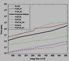

Fig. 5. Computational cost (in seconds) of nine clustering algorithms.
Since, the computational cost above presented is heavily inﬂuenced by the programming style, we also present a quick complexity analysis for all the tested algorithms. Taking into account the time complexity of the original FCM, which is O(nc) is the histogram’s length and is the number of clusters), it is easily deduced that the total complexity of all FCM variations have the same complexity with a small variation depending on the preprocessing step each algorithm uses. On the other hand, the SLINK method has a complexity of O (n2), while the complexity for algorithms FCM_S1, FCM_S2 and the proposed one is O (HWc), where H and W are the dimensions of the image under consideration.

V. CONCLUSION

In this project, a novel robust fuzzy local information c-means (FLICM) algorithm for image clustering was introduced. The proposed algorithm can detect the clusters of an image overcoming the disadvantages of the known FCM algorithms and their variants. This is achieved by incorporating local spatial and gray level information. The FLICM introduces a new factor Gki as a local (spatial and gray) similarity measure which aims to guarantee robustness both to noise and outliers. Also, the algorithm is relatively independent of the type of the added noise, and as a consequence, in the absence of prior knowledge of the noise, FLICM is the best choice for clustering. This is also en- forced by the way that spatial and gray level image information are combined in the algorithm; the factor combines in a fuzzy manner the spatial and gray level information, rendering the algorithm more robust to all kind of noises, as well as to outliers. Furthermore, all the other fuzzy c-means algorithms for image clustering exploit, in their objective functions, a crucial parameter a (or λ), which is used to balance the robustness and effectiveness of ignoring the added noise. This parameter is mainly determined empirically or using the trial-and-error method. The FLICM is completely free of any parameter determination, while the balance between the noise and image details is automatically achieved by the fuzzy local constraints, enhancing concurrently the clustering performance.

VI. REFERENCES

[1] X. Munoz, J. Freixenet, X. Cufi, and J. Marti, ―Strategies for image segmentation combining region and boundary information,‖ PatternRecognit. Lett., vol. 24, no. 1, pp. 375–
392, 2003.
[2] D. Pham, C. Xu, and J. Prince, ―A survey of current methods in medical image segmentation,‖ Annu. Rev. Biomed. Eng., vol. 2, pp. 315–337, 2000.
[3] L. Zadeh, ―Fuzzy sets,‖ Inf. Control, vol. 8, pp. 338–353,
1965.
[4] J. Udupa and S. Samarasekera, ―Fuzzy connectedness and object definition:Theory, algorithm and applications in image segmentation,‖ Graph. Models Image Process. vol. 58, no. 3, pp. 246–261, 1996.
[5] Y. Tolias and S. Panas, ―Image segmentation by a fuzzy
clustering algorithm using adaptive spatially constrained membership functions,‖ IEEE Trans. Syst., Man, Cybern., vol. 28, no. 3, pp. 359–369, Mar. 1998.
[6] J. Noordam, W. van den Broek, and L. Buydens,
―Geometrically guided fuzzy C-means clustering for
multivariate image segmentation,‖ in Proc. Int. Conf. Pattern

Recognition, 2000, vol. 1, pp. 462–465.

[7] M. Yang, Y. J. Hu, K. Lin, and C. C. Lin, ―Segmentation
techniques for tissue differentiation in MRI of ophthalmology using fuzzy clustering algorithms,‖ Magn. Res. Imag., vol. 20, no. 2, pp. 173–179, 2002.

International Journal of Scientific & Engineering Research, Volume 2, Issue 12, December-2011 7

ISSN 2229-5518

[8] G. Karmakar and L. Dooley, ―A generic fuzzy rule based
image segmentation algorithm,‖ Pattern Recognit. Lett., vol.
23, no. 10, pp. 1215–1227, 2002.
[9] M. Ahmed, S. Yamany, N. Mohamed, A. Farag, and T.
Moriarty, ―A modified fuzzy C-means algorithm for bias field estimation and segmentation of MRI data,‖ IEEE Trans. Med. Imag., vol. 21, pp. 193–199,2002.
[10] J. Bezdek, Pattern Recognition With Fuzzy Objective

Function Algorithms.New York: Plenum, 1981.

[11] D. Pham, ―An adaptive fuzzy C-means algorithm for
image segmentation in the presence of intensity
inhomogeneities,‖ Pattern Recognit.Lett., vol. 20, pp. 57–68,
1999.
[12] S. Chen and D. Zhang, ―Robust image segmentation using FCM with spatial constraints based on new kernel- induced distance measure,‖ IEEE Trans. Syst., Man, Cybern., vol. 34, pp. 1907–1916, 2004.
[13] L. Szilagyi, Z. Benyo, S. Szilagyii, and H. Adam, ―MR
brain image segmentation using an enhanced fuzzy C-
means algorithm,‖ in Proc.25th Annu. Int. Conf. IEEE EMBS,
2003, pp. 17–21.
[14] M. Krinidis and I. Pitas, ―Color texture segmentation based-on the modal energy of deformable surfaces,‖ IEEE Trans. Image Process., vol. 18, no. 7, pp. 1613–1622, Jul. 2009. [15] D. Pham, ―Fuzzy clustering with spatial constraints,‖ in Proc. Int. Conf. Image Processing, New York, 2002, vol. II, pp. 65–68.

VII. About the Authors

SANDEEP KUMAR MEKAPOTHULA is working as Assistant Professor in the department of ECE at Rise Groups of Institutions, Ongole, Andhra Pradesh, INDIA. He has received B.Tech, Degree in Electronics and Communication Engineering and currently pursuing

M.Tech at QIS College of Engineering & Technology,
Ongole, Andhra Pradesh, INDIA. His main research interest includes Segmentation, Pattern Recognition and Image Processing.

V. JAI KUMAR is presently working as an Associate Professor in ECE Department, QIS College of Engineering

& Technology, Ongole, India. He
received his B.Tech from JNTU, Hyderabad and M.Tech from Acharya Nagarjuna Univeristy, Guntur, India. He
has seven years of experience of teaching undergraduate students and post graduate students .His research interest are in the areas of image processing and artificial neural networks.