∂yˆ
∂x1
= ∂yˆ
∂x2
= =
∂yˆ
∂xk
= 0 . This point, say -
International Journal of Scientific & Engineering Research, Volume 4, Issue 9, September-2013 2233
ISSN 2229-5518
1Stephen Sebastian Akpan, 2John Usen and 3Thomas Adidaumbe Ugbe
1,2,3Department of Maths/Statistics and Computer Science, University of Calabar, Cross-River State, Nigeria
1steveakpan@yahoo.com,2usen@yahoo.com and 3ugbe_thomas@yahoo.com.
An alternative procedure for solving second-order response surface design problems is proposed in this paper. The method involves the fusion of the Newton-Raphson and the Mean-Centre algorithms to obtain a new procedure for the design problem. The application of this new procedure to second-order response surface design problems gives near-optimal solutions within the optimal region with better precision as compared to the other method.
Process engineers in various industries often desire an optimal setting of yield- influencing factors, which maximize yield. Achieving this with precision requires a coordinated series of designed experiments and subsequent analysis of experimental data. Response Surface Methodology (RSM) is an efficient method (invented by G.E.P Box and K.B. Wilson in 1951) for this purpose. Response Surface Methodology is a collection of mathematical and statistical techniques useful for analysing problems where several factors influence a response variable and the goal is to optimize the response, Montgomery [1]
However, several constraints and impediments can momentarily cause shifts from the optimum. In this event, most process engineers usually “gamble” with factors setting envisaged to be within the optimal region with little or no precision to
ensure near-optimality in their yield. The technique of the RSM for combating this
IJSER © 2013 http://www.ijser.org
International Journal of Scientific & Engineering Research, Volume 4, Issue 9, September-2013 2234
ISSN 2229-5518
pitfall is an unsure process on its own. This research presents a modification of the
RSM procedure for combating this problem with improved precision.
For example, if y is the response variable of a process affected by factors
ξ1 , ξ 2 , ξ 3 , ..., ξ k
assumed continuous and controllable by the process engineer with
negligible error, then RSM is useful for developing, improving and optimizing the response variable. This relationship between the factors and the response variable can
be expressed as
y = f (ξ1 , ξ 2 , ξ 3 , ..., ξ k ) + ε
(1)
Where -
ε~N (0, σ 2 ) are independent statistical errors that represent other sources of
variability not accounted for. If one denotes the expected response by η then the
surface represented by η =
f (ξ1 , ξ 2 , ξ 3 , ..., ξ k ) is a Response Surface.
Modeling most RSM problems is usually difficult since the form of the relationship between the response variable and the factors is usually unknown. Sequel to this, RSM usually starts with finding a suitable approximation for - f . Low order polynomials are used for this purpose as they usually give reasonable approximations for f over a small region of the factors and not the entire space. As a first step, the response is modeled with a polynomial of order one. If well modeled by this, then the
approximating function is called a First-order Model given by
k
y = β0 + ∑ βi ξ i + ε
i =1
(2)
Otherwise and if there is curvature in the system, a polynomial of higher degree such as a Second-order Model is used.
y = β0
k
+ ∑
i =1
βi ξ i
k
+ ∑
i =1
βii
ξ 2 +
∑ ∑
i j
i< j
βij
ξ i ξ j + ε
(3)
Almost all RSM problems utilize one or both of these approximating polynomials. In each model, the levels of each factor are independent of the levels of other factors. In order to get the most efficient result in the approximation of polynomials a proper experimental design must be used to collect data.
A survey of the various stages of development of RSM has been presented in the publication of Khuri and Mukhopadhyay [2]. Their publication gives an organized
coverage of these stages in three eras that describe the evolution of RSM since its
IJSER © 2013 http://www.ijser.org
International Journal of Scientific & Engineering Research, Volume 4, Issue 9, September-2013 2235
ISSN 2229-5518
introduction in the early 1950s. They have described the era, 1951-1975, as one during which the so-called classical RSM was developed. In this era, basic experimental designs for fitting linear response surface models as well as a description of methods for the determination of the optimum operating conditions were developed. They have described the era, 1976-1999, as one in which more recent modelling techniques in RSM including an RSM alternative approach to the Taguchi’s robust parameter design were developed. Finally, the era 2000 (and beyond) has been described as one which will present further extensions and research directions in modern RSM such as discussions concerning response surface models with random effects, generalized linear models, and graphical techniques for comparing response surface designs, etc.
Numerous researchers in various fields have either improved or applied RSM. To mention but a few, Joshi et al. [3] developed an enhanced RSM Algorithm using conditions deflection and second-order search strategies. Wu and Yuan [4] have constructed RS-Designs for qualitative and quantitative factors. Neddermeijer, et al. [5] gave framework for RSM for simulation of optimization models. Adinarayana and Ellaiah [6] used RSM in the optimization of the critical medium components for the production of alkaline Phosphatase by newly isolated Bacilus Sp. J. Pharm. Zangeneh, et al. [7] applied RSM in numerical geotechnical analysis. Gupta and Manohar [8] developed an improved RSM for the determination of failure probability using instance measures. Kawaguk et al. [9] applied RSM in Glucosyltransferase production and conversion of sucrose into Isomaltulose using free Erwinia Sp. cells. Nic Phairiais, et al. [10] used RSM to investigate the effectiveness of commercial enzymes on Buckwheat Malt for brewing purposes. Cook [11] used Genetically Programmed Response Surfaces in optimizing Chip Multiprocessor Designs. Zhang and Gao [12] have applied RSM in medium optimization for Pyruvic acid production of Torulopsis Glabrata TP19 in Batch Fermentation. Ebrahimjsour [13] experimented on a modeling study by RSM and Artificial Neural Network or Culture Parameters Optimization for Thermostable Lipase production from a newly isolated Thermophilic Geobacillus Sp. Strain ARM. Alonzo & Hiroyuki [14] applied RSM in the formulation of nutrient broth systems with predetermined P.H and water activities. Amayo [15] applied RSM to automotive suspension designs. Dayananda et al. [16]
applied RSM in the study of surface roughness in grinding of aerospace materials
IJSER © 2013 http://www.ijser.org
International Journal of Scientific & Engineering Research, Volume 4, Issue 9, September-2013 2236
ISSN 2229-5518
(6061AI-15Vol%SiC25p ). Lenth [17] has reviewed and advanced RSMs in R using RSM updated to version 1.40. Arokiyamany and Sivakumaar [18] used RSM in the optimization process for Bacteriocin. Dutta and Basu [19] used RSM for the removal of Methylene Blue by Acaecia Auricultiformis scrap wood char.
This paper has attempted a development which improves and advances the existing RSM procedure. The improvement aids easy exploration of the optimal region for near-optimal settings that usually become an imperative alternative in the event of not being able to use the actual optimum.
In the build-up of our proposed procedure, we have examined the existing RSM procedure and have identified its major pitfall as the difficulty of exploring near-optimal factors setting. Next is the proposed modification which commences from step seven of the existing procedure. The modification utilizes the fusion of the Newton-Raphson and Mean-centre algorithms respectively for obtaining the optimum and the exploration of near-optimal settings within the optimal region.
The existing RSM procedure is as follows.
1. Plan and run a factorial (or fractional factorial) design around the current operating condition.
2. Fit a linear model (with no interaction or quadratic terms) to the data.
3. Determine the Path of Steepest Ascent.
4. Run tests on the Path of Steepest Ascent until response no longer improves.
5. If curvature of surface is large, proceed to stage six. Else return to stage one.
6. In the neighbourhood of the optimum, design, run and fit a Second Order
Model using Least Squares Technique.
7. Based on the Second Order Model locate optimal setting of the independent variables using Classical Technique.
However locating the optimum setting of the independent variables is just one out of three major processes of the Canonical Analysis procedure of the RSM. The
other two aspects include:
IJSER © 2013 http://www.ijser.org
International Journal of Scientific & Engineering Research, Volume 4, Issue 9, September-2013 2237
ISSN 2229-5518
(i) Characterizing the obtained optimal setting of stage seven. That is, explaining
the ridge systems.
(ii) Explaining the relationship between the canonical variables - {wi }
and the
design variables - {xi }. This aspect aids the exploration of the optimal region for near-optimal settings.
Using the existing RSM approach, if one desires to find the levels of
x1 , x2 , x3 , xk
that maximize the expected response - yˆ , the maximum point if it
exists will be the set of
x1 , x2 , x3 ,, xk
such that the partial derivatives -
∂yˆ![]()
∂x1![]()
= ∂yˆ
∂x2
= =
∂yˆ![]()
∂xk
= 0 . This point, say -
x10 , x20 , x30 ,, xk 0
is called the Stationary
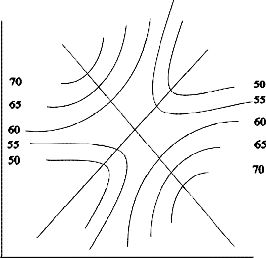
Point. The stationary point could represent (a) a point of maximum response (b) a point of minimum response (c) a saddle point. The figure below shows these three possibilities.
IJSER © 2013 http://www.ijser.org
International Journal of Scientific & Engineering Research, Volume 4, Issue 9, September-2013 2238
ISSN 2229-5518
x2 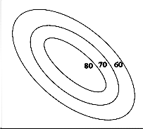
x1
(a )
x2 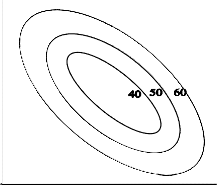
x1
(b)
x2
x1
(c)
FIGURE – Stationary Points in a Fitted Second-Order Response Surface (a) Maximum Response (b) Minimum Response (c) Saddle Point
The existing RSM approach obtains a general solution for the stationary point as follows.
We write the Second-order Model in matrix notation as
IJSER © 2013 http://www.ijser.org
International Journal of Scientific & Engineering Research, Volume 4, Issue 9, September-2013 2239
ISSN 2229-5518
yˆ = βˆ + x
T b + x
T Bx
(4)
Where
x
βˆ
βˆ![]()
βˆ 2
![]()
βˆ 2
![]()
βˆ 2
1
1
11 12 13
1k
x2
βˆ
ˆ22 β 23 2 ˆ2 k
, b = βˆ
and
βˆ
βˆ 2
3
3
33 3k
ˆ ˆ
xk
β k
sym.
β kk
That is, b is a (k ×1)
vector of the first-order regression coefficients and B is a
(k × k )
symmetric matrix whose main diagonal elements are the pure quadratic
coefficients {βˆ }
and whose off-diagonal elements are one-half of the mixed
quadratic coefficients - (βˆ
equated to zero is
, i ≠
j ). The derivative of yˆ with respect to the vector x
∂yˆ![]()
∂x
= b + 2Bx = 0
(5)
The stationary point is the solution to Equation (5), or![]()
0 2
(6)
Furthermore, by substituting (6) into (4) we can find the expected response at
the stationary point as
yˆ = βˆ
![]()
+ 1 x T b
(7)
0 0 2 0
Using the existing RSM procedure ultimately requires the conversion of points in the {wi }-space to points in the {xi }-space in other to explore the optimal region for near-optimal factors setting. How can one precisely select points in the {wi }-space if
not by gambling or intuition based on experience? More so, the selected points in the
{wi }-space are converted to points in the {xi }-space using the canonical equation that
IJSER © 2013 http://www.ijser.org
International Journal of Scientific & Engineering Research, Volume 4, Issue 9, September-2013 2240
ISSN 2229-5518
has no unique solution. This procedure of the RSM invariably implies that the process engineer can only but gamble with options of near-optimal factors settings should it become difficult to operate at the optimum operating condition owing to machine deterioration, drop in machine efficiency, voltage fluctuations, etc. This process of gambling is often time-consuming and does not guarantee precision in the selection of near-optimal factors settings. There is therefore an imperative need for the advancement of the existing RSM procedure to curb this problem. We have perused several literatures on different research directions with which several authors have either applied or advanced the RSM procedure, none of which has made an attempt to curb this problem using our proposed research direction.
To advance the existing RSM procedure we proffer the following procedure that continues from stage seven of section cited above. Rather than using the existing RSM procedure of the classical derivative technique for locating the optimum as cited in stage seven, we shall be using the Newton-Raphson iterative algorithm to locate the optimum. We shall call this step our step eight.
8. Based on the Second Order Model locate the optimal setting of the independent variables using the Newton-Raphson algorithm below (with the design centre as our initial approximation). Using the design centre as our initial approximation, this algorithm terminates after one iterate or one more.
9. Find near-optimal factors settings using the Mean-Centre algorithm below.
Step 1: Input
x 0 in the function - f (x t ). Put - t = 0 .
Step 2: Evaluate -
f (x t ). Test for end of optimization. If E t
has not increased
over a number of iterates, terminate the maximization and set -
Else return to step three.
Step 3: Evaluate the Jacobian gradient g t
at the point - x t .
IJSER © 2013 http://www.ijser.org
International Journal of Scientific & Engineering Research, Volume 4, Issue 9, September-2013 2241
ISSN 2229-5518
∂f (x t )
![]()
∂x1
∂f (x t )
![]()
∂x
2 ![]()
g t = ∇f (x t ) = ∂f (x t )
∂x3
∂f (x )
t
∂xn
Step 4: Compute the Hessian H t
and its inverse
t at - x t .
![]()
∂ f (x t )
2
![]()
∂f (x t )
∂x1
∂x1∂xn
∂f (x t )
∂f (x t )
![]()
∂x ∂x ![]()
∂x 2
n 1 n
Step 5: Compute the direction of improvement - U t
= ∆x t
![]()
![]()
= t t .
t t
![]()
![]()
![]()
(x∗ )2 + (x∗ )2 + (x∗ )2 + + (x∗ )2
t t 1 2 3 n
Step 6: Find the optimum step length λt
in the direction - U t .
Step 7: Generate new point.
= x t
+ λt U t
= x t
+ λt
−1
t t
![]()
![]()
t t
Replace t by t + 1 and return to step two. Else, set x t
to step eight.
as optimal setting and proceed
Step 8: Input
x 0 = (x01 , x02 , x03 ,, x0 n ) and x
= (x , x , x ,, x )
∗ ∗ ∗ ∗ ∗
n
Step 9: Evaluate x
t +1
= t
2
at t = 0
Step 10: Evaluate
f (x t +1 ) at t = 0
IJSER © 2013 http://www.ijser.org
International Journal of Scientific & Engineering Research, Volume 4, Issue 9, September-2013 2242
ISSN 2229-5518
Step 11: If
f (x
t +1
) < f (x∗ )
increase t by 1 and go to step nine. Else, set
= x∗ if
f (x
t +1
) = f (x∗ )
A modification of the existing Response Surface Technique has been proposed for solving Second-Order Response Surface Design Problems. It comprises a fusion of two iterative techniques (Newton-Raphson algorithm and Mean-Centre algorithm). The improvement unravels the design centre in the optimal region as a good initial approximation for starting the Newton-Raphson iteration; it also affords process engineers the liberty of exploring near-optimal operating conditions.
[1] D. C. Montgomery, “Regression Analysis and Response Surface Methodology”.
Design and Analysis of Experiments pp. 305-368. New York: John Wiley & Sons. Website: http://www.stat.purdue.edu/~bacraig/note1/topic26.pdf),1995.
[2] A. Khuri and S.Mukhopahyay, “Response Surface Methodology.” Wiley
Interdisciplinary Reviews, Computational Statistics, Vol. 2, Issue 2, pp. 128-
149).NewYork:JohnWiley&Sons,Inc.,Website:http://onlinelibrary.wiley.com/do i/10.002/wics.73/abstract),2010
[3] S. Joshi, H. D. Sherali and J. D. Teu, “ An Enhanced Response Surface Methodology (RSM) Algorithm Using Conditions Deflection and Second-Order Search Strategies.” Computers and Operations Research. 25 (7/8), pp.531-
541,1998
[4] C. F. J. Wu and D. Yuan, “Construction of Response Surface Designs for
Qualitative and Quantitative Factors.” IIQP Response Report RR-91-03
Website:http://www.sciencedirect.com/science/article/pii/50378375898000032,
1998
[5] H. G. Neddermeijer, G. J. Van Oortmarssen, N. Piersma and R. Dekker, “A Framework for Response Surface Methodology for Simulation Optimization
Models.” Proceedings of the 2000 Winter Simulation, pp. 129-136 ,2000
IJSER © 2013 http://www.ijser.org
International Journal of Scientific & Engineering Research, Volume 4, Issue 9, September-2013 2243
ISSN 2229-5518
[6] K. Adinarayana and O. Ellaiah, “Response Surface Optimization of the Critical Medium Components for the Production of Alkaline Phosphatase by Newly Isolated Bacilus Sp”, J. Pharm. Pharmaceut. Sci 5(3) 272-278,2002.
[7] N. Zangeneh, A. Azizian, L. Lye and R. Popesiu, “Application of Response Surface Methodology in Numerical Geotechnical Analysis.” 55th Canadian Society for Geotechnical Conference, Hamiltons, Ontario, 2002. Canada: University of New Found Land; St. John’s, NF. Website: http://www.engr.nun.ca/~llye/RSM-Geotech.pdf ,2002
[8] S. Gupta and C. S. Manohar, “An Improved Response Surface Method for the
Determination of Failure Probability and Using Instance Measures,”pp. 123-
139India:ElsevierLimited.Website:http://civil.iisc.ernet.in/manohar/%sayanmao har.pdf,2003
[9] H. Y. Kawaguk, E. Manrich and H. H. Sato, “Application of Response Surface Methodology for Glucosyltransferase Production and Conversion of Sucrose into Isomaltulose Using Free Erwinia Sp. Cells,” Electrical Journal of Biotechnology,Vol.9,No.5.Website:http://www.ejbiotechnology- info/content/Vol9/issue5/full/6,2006.
[10] P. B. Nic Phairiais, B. D. Schela, J. C. Oliverta and E. K. Arendt, “Use of Response Surface Methodology to Investigate the Effectiveness of Commercial Enzymes on Buckwheat Malt for Brewing Purposes.”Journal of the Institute of Brewingpp.324-332,
Website:http://www.scientificsocieties.org./job/papers/2006/G2006-1308-
459.pdf
[11] H. Cook, “Optimizing Chip Multiprocessor Designs Using Response Genetically![]()
Programmed Response Surfaces,” A Thesis in STS402. University of Virginia: Faculty of the School of Engineering and Applied Science,2007
[12] J. Zhang and N. Gao, “Application of Response Surface Methodology in Medium Optimization for Pyruvic Acid Production of Torulopsis Glabrata TP19 in Batch Fermentation.” Journal of Zhejiang Universiity of Science, pp 98-
104,2007.
IJSER © 2013 http://www.ijser.org
International Journal of Scientific & Engineering Research, Volume 4, Issue 9, September-2013 2244
ISSN 2229-5518
[13] A. Ebrahimjsou, R. N. Rahman, H. D. Eanchng, M. Basri and A. B. Salleh, “A Modeling Study by Response Surface Methodology and Artificial Neural Network or Culture Parameters Optimization for Thermostable Lipase Production from a Newly Isolated Thermophilic Geobacillus Sp. Strain ARM. BMC.”BiochemistryWebsite:http://www.biomedcentral.com/1472-
6750/8/90,2008
[14] A. G. Alonzo and N. Hiroyuki, “Application of Response Surface Methodology in the Formulation of Nutrient Broth Systems with Predetermined P.H and Water Activities. African Journal of Microbiology Research,” Vol.45,No.2,pp.634-639,AmericanSocietyforMicrobiology,
Website:http://www.ncbi.nlm.nih.gov/pmc/articles/PMC2425361,
[15] T. Amayo, “Response Surface Methodology and its Application to Automative
SuspensionDesigns” Website:http://www.personal.umich.edu/~kikuchi/Research/rsmamayo.pdf,2010.
[16] R. Dayananda, R. Shrikantha, S. Raviraj and N. Rajesh, “Application of Response Surface Methodology on Surface Roughness in Grinding of Aerospace Materials (6061AI-15Vol%SiC25p ).” ARPN Journal of Engineering and Applied Science Vol. 5, No. 6 Asian Publishing Network (ARPN). Website: http://www.arpnjournal.com,2010.
[17] R. V. Lenth, “Response-Surface Methods in R, Using rsm”, The University of
Iowa,Website:http://eran.r.project.org/web/packages/rsm/rignettes/rsm- pdf,2010.
[18] A. Arokiyamany and R. K. Sivakumaar, “The Use of Response Surface Methodology in Optimization Process for Bacteriocin.” International Journal of BiomedicalResearch,Vol.2,No.11.Website: http://ssjournals.com/index.php/ijbr/ksw/Arokiyamany,2011.
.
IJSER © 2013 http://www.ijser.org
International Journal of Scientific & Engineering Research, Volume 4, Issue 9, September-2013
ISSN 2229-5518
2245
[19] M. Dutta and J. K. Basu, "Response Surface Methodology for the Removal of Methylene Blue by Acaecia Auricultiformis Scrap Wood char." Research Journal of Environmental Toxicology, Vol. 5, Issue 4/ pp. 265-278, Website: http://scialert.net/abstract/?doil=rjed. 2011.266.278,2011.