International Journal of Scientific & Engineering Research, Volume 4, Issue 7, July-2013 2453

ISSN 2229-5518

Aerodynamic Exterior Body Design of Bus

A.Muthuvel1, M.K.Murthi2, Sachin.N.P3, Vinay.M.Koshy4, S.Sakthi5, E.Selvakumar6

[1 Department of Automobile Engineering,Hindustan University, India

2-6 Department of Mechanical Engineering, Nandha Engineering College,India]

Abstract— The rising fuel price and strict government regulations makes the road transport uneconomical now a days. The exterior styling and aerodynamically efficient design for reduction of engine load which reflects in the reduction of fuel consumption are the two essential factors for a successful operation in the competitive world. The bus body building companies’ precedence’s are outer surface and structure of the bus and ignore the aerodynamic aspect. The present intercity buses have a poor aerodynamic exterior design. The overall aim of this project is to modify the outer surface and structure of the bus aerodynamically in order to reduce the effect of drag force of the vehicle which in turn results in reduction of fuel consumption of the vehicle. Experimental and numerical tests have been conducted in Wind Tunnel to prove the effectiveness of the new concept design. It is evident from the test result, that there has been a considerable reduction in drag force of about 30%-34% from the existing bus to the new concept and 6 to 7 litres of fuel is consumed for the every

100Km.

Index Terms— Bus body, CFD analysis, Drag reduction, Exterior aerodynamics, , Fuel, consumption, W ind tunnel test.

——————————  ——————————

1 INTRODUCTION

he rise in the deterioration of fossil fuel is one of the most critical dilemmas which the world will face in the imminent decades. Petroleum products account to 40%
of the total amount of fossil fuels. Diesel and gasoline are the vital petroleum products, which are disintegrated day by day. Out of the total petroleum products consumed by various sectors, 66% of i`t is consumed for transportation.
Buses are major means of mass transportation in India. Indian road have been significantly improving for the past
10years and the travel time have been reduced as they can travel with high speeds. Therefore, it has become crucial to engender buses with better fuel efficiency. Stringent government regulation and rising fuel prices has forced the vehicle manufacturers to produce fuel efficient buses. The bus body manufacturers in India are concern only about the aesthetic sense of buses. They give least importance to aerodynamics and its affect in fuel consumption of high speed moving buses.
In a moving vehicle, the engine power is used to overcome tractive resistance, which is the combination of rolling and aerodynamic resistance. The rolling resistance will be dominant over the aerodynamic resistance at lower speeds. But as the speed of the vehicle increases, the aerodynamic resistance dominates the rolling resistance. Thus, reducing the aerodynamic resistance at high speed, the load on the engine which in turn boosts the fuel efficiency of the bus gets reduced.
Edwin J Saltzman [1] carried out studies on reducing the drag of trucks and buses their final model equipped with rounded horizontal and vertical corners, smoothed under body and a boat tail achieved the required drag coefficient. The NASA Dryden Flight Research Center test van, a box-shaped ground vehicle with a truncated boat tail after body, has achieved an aerodynamic drag coefficient of
0.242. This drag coefficient is slightly lower than the trucking industry and U. S. Department of Energy goal of
0.25. Ludovico Consano [2] at IVECO truck building company came up with an aerodynamically efficient truck. They paid particular attention on the corner surfaces of the vehicle. Moreover the lateral lowered side skirts have been added to mask the tanks, rear wheels and axles. To prevent flow detachment, many rounded surfaces have been added to the exposed surfaces, such as the roof window, side mirrors, sun visor, etc. The test results revealed a fuel reduction of 8%.R. Mc Callen, et al [3] in their experiments found out removal of rear view mirror alone will bring down the drag of the vehicle by 4.5%. Any gap in the vehicle body will result in flow separation and flow circulation. Gilhaus [4] Investigation revealed a reduction in drag value until the front leading edge radii value reaches 150 mm. Further increase in the radius did not affect the drag value of the bus. G W Carr [5] investigated the effects of streamlining the front end of the rectangular bodies in ground proximity. Experiments shown a stream lined front end with low leading edge resulted in a drag coefficient of 0.21. W.H.Hucko [6] and H J Emmelmann [7] found that detailed shape optimization of parts such as roof radii, rain channels, headlights will result in reduction of drag force.
The overall aim of our project is to redesign an intercity
bus with enhanced exterior styling and reduced
aerodynamic resistance which could provide better fuel efficiency.

2 DIMENSIONAL SPECIFICATION

As the existing bus has a flat front it has more resistance to air and hence the drag force is very high and the stability is also very low at higher speed. In order to overcome these problems, we have come up with our exterior body design keeping the existing model as benchmark. Here we have made four models each having different exterior body styling and appearance.

IJSER © 2013 http://www.ijser.org

International Journal of Scientific & Engineering Research, Volume 4, Issue 7, July-2013 2454

ISSN 2229-5518

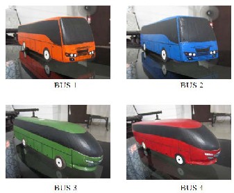
Here we have designed four different buses, in order to optimize the contribution of each modification on the drag force. The first bus is the existing bus. The second bus has side tapering towards the rear end to provide better streamlined flow. The third bus has an aerodynamically shaped front with front spoiler and the remaining is same as that of first bus. The fourth bus has as aerodynamically shaped front with front spoiler. It also has a side and roof tapering towards the rear end are shown in Figure 1.

Fig. 1. Bus Prototypes

3 EXPERIMENTAL RESULT (WIND TUNNEL TEST)

The Wind Tunnel analysis of flow over the bus is made for various speeds with all the buses. Drag forces are measured for various speeds from 80 to 115 kmph with an increment of 5kmph. The percentage of drag deviation between the bus 1 and bus 4 is 20%, 16%, 21%, 31%, 29%,
35%, 31%and 30% for different speeds from 80 kmph to
115kmph. The drag force for the speed of 80-115 kmph is
shown in Table1.
The deviation of drag force of second bus with respect
to the first bus will give a clear idea about how much the
drag force is affected by the rear modification. The
deviation of drag force of third bus with respect to the first
bus will give a clear idea about how much the drag force is
affected by front modification. The deviation of drag force of fourth bus with respect to the first bus will give a clear idea about how much the drag force is affected by the overall modification.

4 ANALYTICAL RESULTS AND ANALYSIS OF BUS

Three dimensional numerical analysis of the flow over Autonomous Under-Water Vehicle (AUV) is carried out with the general purpose Reynolds Averaged Navier- Stokes Equations (RANSE) solver STAR-CCM+. Steady analysis is carried out both with unstructured polyhedral mesh with AKN k-ε model turbulence models for bus1-bus4. For all the cases, the maximum residual from continuity, x-momentum, y-momentum and z-momentum is restricted to 10-6 as convergence criteria. Initially, 300 iterations are carried out with first-order upwind scheme and relaxation factor for velocity as 0.3 and pressure as 0.1 to guard against divergence of the solution. Later, till the convergence criteria are met, iterations are carried out with second-order upwind scheme with velocity relaxation factor as 0.5 and pressure relaxation factor as 0.3 to obtain higher accuracy and also to accelerate the convergence.

4.1 Geometrical Modelling

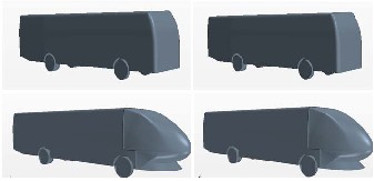
Scaled 1:30 three dimensional AL PSV 4/157 CAD models of buses Bus 1 to Bus 4 are shown in Figure 3 by using the Solid works CAD software with its actual dimensions are shown in Table 2.

TABLE 1

DRAG FORCE FOR VARIOUS SPEEDS

IJSER © 2013 http://www.ijser.org

International Journal of Scientific & Engineering Research, Volume 4, Issue 7, July-2013 2455

ISSN 2229-5518

TABLE 2

BUS SPECIFICATIONS

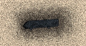
Fig. 4. Sectional view of bus 4 and domain with unstructured mesh

4.3 Boundary Conditions

Boundary conditions were applied on the meshed model using the STARCCM+ CFD software. The analysis was carried out in moving road and rotating wheel condition. In the simulation only straight wind condition was considered at 3 different vehicle speed of 80, 100,115
Km/hr. Constant velocity inlet condition was applied at the

inlet to replicate the constant wind velocity conditions same
as wind tunnel tests. Zero gauge pressure was applied at
the outlet with operating pressure as atmospheric pressure. All the boundary conditions used in the analysis are listed in Table 3.

TABLE 3

BOUNDARY CONDITIONS

Fig. 2. Geometrical modelling of Bus 1 – Bus 4

4.2 Grid Generation

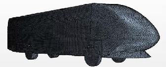
Unstructured polyhedral mesh is chosen while generating the grid. During generation of the meshes, attention is given for refining the meshes near the bus so that the boundary layer can be resolved properly. The typical mesh for bus 4 is shown in Figure 3 and a magnified view near the solid wall of bus 4 is shown in Figure 4

4.4 Results For Unstructured Mesh

Fig. 3. Bus 4 with unstructured polyhedral mesh

Grid independent test is carried out for all the buses from 0.74 million to 2 million cells. AKN k-ε two layer models were used for the test. The drag coefficient values along the surface of the bus against the experimental values. From Table 4 it can be seen that the values at 1.15 million and 1.31 million cells are deviating very much from the values obtained with 1.57 million cells. However, difference between the values obtained from 1.31 million cells with those 1.57 million cells is very less (less than 5%).

IJSER © 2013 http://www.ijser.org

International Journal of Scientific & Engineering Research, Volume 4, Issue 7, July-2013 2456

ISSN 2229-5518

TABLE 4

GRID INDEPENDENT TEST

Hence, 1.57 million cells are considered for further analysis for Bus 1.
The CFD analysis of flow over the bus is made for various speeds with all the buses. Drag force is measured for various speeds like 80,100 and 115 kmph. The drag coefficient is derived from drag force. The percentage of drag deviation between the bus 1 and bus 4 is 34%, 30% and 31 % for the speed of at 80kmph, 100kmph and
115kmph. By the 30-34 % drag deviation we can able to
reduce the huge amount of fuel consumption. The drag
coefficient for the speed of 80-115 kmph is shown in Table
5-7.

TABLE 6

COMPARISONS OF RESULTS AT 100 KMPH

TABLE 5

COMPARISONS OF RESULTS AT 80 KMPH

TABLE 7

COMPARISONS OF RESULTS AT 115 KMPH

IJSER © 2013 http://www.ijser.org

International Journal of Scientific & Engineering Research, Volume 4, Issue 7, July-2013 2457

ISSN 2229-5518

5 CALCULATION OF FUEL CONSUMPTION

The fuel consumption of the bus at various speeds is calculated with the help of a tool, named “Aerodynamic and Rolling Resistance, Power and MPG calculator”, (http://ecomodder.com/forum/tool-aero-rolling- resistance.php). The result may not be authentic. Aerodynamic, rolling, and acceleration resistances are assumed to be the only resistive forces acting against the vehicle motion.
For calculating the fuel consumption, values of the
following particulars of the vehicle have been entered.

TABLE 8

PARTICULARS FOR CALCULATING FUEL CONSUMPTION

The calculated fuel efficiency of all the four buses at three different speeds are tabulated below.

TABLE 8

FUEL CONSUMPTION PER 100KM

tested for optimizing how each modification is contributing towards the drag force. The experimental test which we have conducted gives us a clear idea that there has been a considerable reduction of drag force on the models which we have created. It was found that the least drag force was acting on Bus No.4. The Bus No.2 and Bus No.3 gave an intermediate result as expected. The percentage reduction in drag force of Bus No.4 from Bus No.1 is found to be 30%-
34%.By the 30-34% deviation in drag force, fuel consumption of about 8% to 23% can be reduced from 80 kmph to 115 kmph. This improvement in fuel efficiency
will have a high impact on the reduction of annual fuel consumption. Hence the aim has been achieved.

REFERENCES

[1] Edwin. J. Asltzman and Robert. R. Meyer., (1999), “A reassessment of heavy duty truck aerodynamic design features and priorities”, NASA/tp-1999-206574.

[2] Mr.Ludovico Consano and Davide Lucarelli., (2007), “Fuel Reduction on a Tractor-Trailer Truck at IVECO IVECO S.p.A”, 3 rd European automotive CFD conference, EACC 2007.

[3] R.Mc. Callen, K. Salari, J. Ortega, F. Browand, M. Hammache, T.

Hsu., (2004), “Effort to Reduce Truck Aerodynamic Drag – Joint Experiments and Computations Lead to Smart Design”, AIAA Fluid Dynamics Conference, June 28 – July 1.

[4] Gilhaus A., “Main parameters determining the aerodynamic drag of

buses, colloque construire avec le vent, vol 2.

[5] Carr.G.W., (1982), “The aerodynamics of basic shapes of road vehicles, part 1, Simple rectangular bodies”, MIRA report No.1982/2.

[6] Wolf Heinrich Hucho., (2001), “Aerodynamics of road vehicles”, 4th

edition, SAE International, vol.1, pp. 11-88.

[7] Hucko,W.HEmmelmann. H.J (1977) “Aerodynamiche Formoptimierung,ein weg zur steigerung der wirtschsftlichkeit von nutzfahrzeugen,” Series.12, NO.31 1977.

6 CONCLUSION

Four different prototypes have been fabricated for performing experimental and numerical analysis using wind tunnel and CFD software. The Bus No.1 is the existing model, Bus No.2 is the existing model with the rear end modified, Bus No.3 is the existing bus with the front end modified and Bus No.4 is the model with modification at front and rear end. The four models have been separately

IJSER © 2013 http://www.ijser.org