International Journal of Scientific & Engineering Research, Volume 2, Issue 1, January-2011 1

ISSN 2229-5518

A Role of Query Optimization in Relational

Database

Prof.M.A.Pund, S.R.Jadhao, P.D.Thakare

Abstract— Nowadays, we are flooded with information through and from the Databases. We have to deal with a constantly increasing amount of facts, figures and dates. Therefore, it is necessary to somehow store this information in an adequate way. This is what database systems were developed for. One particular approach is the relational databases. In a relational database all information can be found in a series of tables in which data is stored in rows and columns. The problem with SQL query, its declarative – does not specify a query execution plan and also we have to deal with as a consequence is the question as how to find the specific facts that might interest us amongst all the information stored in the described tables. And as one might put it, “Time is Money” in our society, it is not only important to find the required information, but also with proper execution plan so that it takes less time. The solution is to convert SQL query to an equivalent relational algebra and evaluates it using the associated query execution plan.

This paper will introduce the reader to the basic concepts of query processing and query optimization in the relational database domain. How a database processes a query as well as some of the algorithms and rule-sets utilized to produce more efficient queries will also be presented. I will discuss the implementation plan using join orderingto extend the capabilities of Database Engine program through the use of randomized algorithms iterative improvement method in the database area in the context of query optimization. More specifically, large combinatorial problems such as the multi-join optimization problem have been the most actively applied areas [9].

Index Terms—SQL Query optimization, relational database, Query Processing

1. INTRODUCTION

—————————— • ——————————
Query optimization plays a vital role in query processing. Query processing consists of the following stages:
1. Parsing a user query (e.g. in SQL)
2. Translating the parse tree (representing the query) into relational algebra expression.
3. Optimizing the initial algebraic expression.
4. Choosing an evaluation algorithm for each rela-
tional algebra operator that would constitute
least cost for answering the query.
Stages 3-4 are the two parts of Query Optimization. Query optimization is an important and classical compo- nent of a database system. Queries, in a high level and declarative language e.g. SQL, which require several al- gebraic operations, could have several alternative compo- sitions and ordering. Finding a “good” composition is the job of the optimizer. The optimizer generates alternative evaluation plan for answering a query and chooses the plan with least estimated cost. To estimate the cost of a plan (in terms of I/O, CPU time, memory usage, etc but not in pounds or dollars) the optimizer uses statistical information available in the database system catalogue [5].

2. QUERY OPTIMIZATION

2.1 What is a Query: A First Approach?

In a relational database all information can be found in a
series of tables. A query therefore consists of operations on tables. Here a list of the most commonly performed operations:
• Select (o): Returns tuples that satisfy a given predicate
• Project (rr): Returns attributes listed
• Join (): Returns a filtered cross product of its argu-
ments
• Set operations: Union, Intersect, and Difference
The most common queries are Select-Project-Join queries.
In this paper, we will look at queries, which consist of
these three operations on tables only, focusing on the join-
ordering problem we will see in the following example.

2.2 Example

To illustrate how a query is performed and why query optimization might be necessary, we will look at the fol- lowing basic database:

Student: { stud_id, name, semester } Lecture: { lect_id, title, lecturer } Professor: { prof_id, name } Enrolment: { stud_id, lect_id }

The question we want to ask is:
Which semester are the students in, which are enrolled in
a course of professor Newton?
If we translate this into an SQL query, in a first step, we
might get:

Select distinct s.semester

From student s, professor p, enrolment e, lecture l

Where p.name = ‘Newton’ and

IJSER © 2010 http://w w w .ij ser.org

International Journal of Scientific & Engineering Research, Volume 2, Issue 1, January-2011 2

ISSN 2229-5518

l.lecturer = p.prof_id and l.lect_id = e.lect_id and e.stud_id = s.stud_id
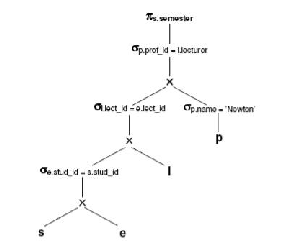
This query gives us the following access plan:
We see very quickly that this query cannot be the best
way to reach our answer. We have three cross products, which means that we create a table whose number of rows is |s|*|e|*|l|*|p|. For large tables s, e, l and p this result is not acceptable.
One possible way of improving this is to perform the se- lections (here done in the very last step) earlier on in the search as shown in Fig.1.
This way, we get the following result:
ordering we use. [5].
To illustrate this, we look at an example:
We consider the three relations S, R and T as shown in
Table 1, 2, 3.
Each one of the tables consists of a number columns
and rows. By illustrating the join procedure for the cases (RS) T or R (ST), we will see, why the join or- dering does indeed matter. The result of these operations
will be the same, as expected. But we will see, that the tables produced at the intermediate step will vary consi- derably with regards to their size:
TABLE 1 TABLE 2 TABLE 3
Relation R Relation S Relation T

Fig.1. Query Plan 1

By doing the selections earlier on, we make restrictions
and our final table is of smaller size than the former one.
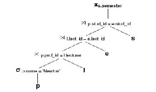
We can improve our result even more by substituting the
cross with join operators as shown in Fig.2.
The result is:
Case 1 : (RS) T
TABLE 4

Result of (RS)


TABLE 5
Result of (RS) T

Fig.2. Query Plan 2

Case 2: R (S T)
TABLE 6

Result of (S T)
We have improved our original query model. But now we are at a point were it gets harder to tell how to further improve our model: Knowing that the join operator is commutative as well as associative, we don’t know which order of these joins would suit us best to minimize the resulting table at each step. Even though the result of the joins will be the same, it makes a difference, which join

TABLE 7
Result of R (S T)
IJSER © 2010 http://w w w .ijser.org

International Journal of Scientific & Engineering Research, Volume 2, Issue 1, January-2011 3

ISSN 2229-5518

We see that in the first case, a temporary relation with many rows has to be stored as shown in Table 4 even though it is reduced to only one row as shown in Table 6 in the second step.
In the second case, however, we have chosen a better join ordering. The temporarily stored relation contains only one row. Hence, the great importance of the join ordering is notified.

2.3 Some Definitions and Terms

In this elaboration, we will use following notations:
In query optimization we are looking at a state space con-
sisting of all access plans that compute the same result to a
query.A solution of any given problem is described in a

processing tree.

Every one of the access plans is associated with a certain

cost, which is given by a cost function. I will not introduce

exact cost models in this elaboration. For now we just assume, that the cost function usually takes as input the number of pages that have to be read from or written to secondary memory to calculate a cost estimate for the
access plan.
If the database is assumed to be much larger than the
available memory, we can neglect al costs except for the
I/O costs. The processing tree is, as we have encountered
it in the previous chapter, a binary tree. It consists of
leaves that are the base relations, internal nodes which are
the join operators and edges, which represent the data
flow [8],[ 9].
All possible access plans to a query define our state space E.This state space might become very large, for some cas- es. Therefore, we might choose to simplify it and reduce the amount of access plans by only allowing access plans
of a certain shape.
In general, a node in a processing tree can have operands,
which are composites themselves. This is what we call a

bushy tree. If we want to form a binary tree out of n base

relation (all of which can figure only once in the


minim- al cost access plan is called an optimal solution to the query.

3. QUERY OPTIMIZATION ALGORITHMS: AN OVERVIEW

When developing query algorithms, the optimality of the produced access plans is a very important issue. There- fore, many different algorithms have been developed and proposed as a good approach to the query optimization problem. So far, all of these algorithms can be divided into three major categories:
1) Deterministic Search Algorithms
2) Genetic Algorithms
3) Randomized Algorithms

Evaluation:

In Deterministic Search Algorithms:-On the other hand, it
is known that the dynamic programming algorithm has
high memory consumption for storing all the partial solu-
tions found in the different loops.
Another downside of dynamic programming is its expo-
nential running time. This makes an application involving
more than about 10 – 15 queries prohibitively expensive.
Still, for queries with only a few joins, this approach
works very well.
In Genetic Algorithms:- A problem with this approach
might be that one member of the population is so promi-
nent that it dominates the whole wheel. This way, it caus- es the disappearance of the other members’ features. The evolution converges toward a generation, consisting of one super member. Even if the extinct members of the
population might not have provided a high quality solu- tion, they could still contain some valuable information. Randomized algorithms are based on statistical concepts where the large search space can be explored randomly using an evaluation function to guide the search process closer to the desired goal. Randomized algorithms can find a reasonable solution within a relatively short period of time by trading executing time for quality. Although

processing tree) we find ( n 2 ( n 1) 1)( n 1)!

different
the resulting solution is only near-optimal, this reduction
solutions. This means that the state space becomes very
large for growing n. A common restriction that is often
made to reduce the size of the state space, is to allow only so called linear trees. A linear tree is a tree, whose internal nodes all have at least one leaf as a child. To take this even further, many algorithms consider only the space of
all left-deep trees, meaning that only trees of the follow- ing form are allowed.This restriction reduces the number of accepted access plans significantly. The set of all possi- ble left-deep access plans with n base relations is reduced to n! [3].

2.4 Formal Approach

With the notations given above, we can attempt to state the general problem of query optimization as follows: Given a query q, a space of access plans E, and a cost function cost(p) that assigns a numeric cost to an execution plan p€E. Find the minimum cost access plan that computes q. This
is not as drastic as the reduction in execution time. Usual- ly, the solution is within a few percentage points of the optimal solution which makes randomized algorithms an attractive alternative to traditional approaches [6],[7].

3.1 Randomized Algorithms

The problem of finding an optimal plan is NP hard. Therefore we might try, if randomized algorithms could improve our search of an optimal plan.
A randomized algorithm is an algorithm that makes ran- dom choices as it proceeds. In our case, this means, that the algorithm performs random walks in the state space. Itmoves from state to state with the goal of finding a state with the minimum cost [1],[5],[6].
The advantages of randomized algorithms:
- Simplicity: There are many examples, where a rando- mized algorithm can match or even outperform a deter- ministic algorithm
- Speed: There are cases where the best known rando-
IJSER © 2010 http://w w w .ij ser.org

International Journal of Scientific & Engineering Research, Volume 2, Issue 1, January-2011 4

ISSN 2229-5518

mized algorithm runs faster than the best known deter- ministic algorithm.
_ Lower time bounds are expected in many cases.
Possible inconveniences of randomized algorithms:
- Often, the required solution is found only with high probability
- A randomized algorithm might not find the correct an- swer at all [1].
- There might exist cases, where a randomized algorithm could take very long to find the correct answer.
In the following sections, The best known randomized algorithm, As per study,I will suggests the randomized because this is the only approach which is better suited for join optimizations.
Which again are two different randomized algorithms named Iterative Improvement (II) and Simulated Anneal- ing (SA).
But for a start I will start with Iterative Improvement me-
thod; it will be necessary to introduce some terminology
which is commonly used when working with randomized
algorithms [1].

3.1.1 Terminology

Randomized algorithms consider access plans as points in the solution space.
Different access plans are connected through edges, allow- ing us to move around the solution space. These edges are defined by a set of allowed moves.
This set depends very much of the solution space. A commonly used set for left-deep processing trees would for example be the following:
S = {Swap, 3Cycle}, where swap simply exchanges the positions of two arbitrary relations and 3Cycle performs a cyclic rotation of three arbitrary relations in the processing tree (Note that this is allowed due to the commutativity and associativity of the join operator.) Neighbour(A) is the set of access plans that can be reached from the access plan A by performing moves defined in S. Further, we call a state A a local minimum if for paths starting at A any downhill move comes after at least one uphill move, whereas a state is considered to be a global minimum if it has the lowest cost among all states in the solution space[2].

3.1.2 Iterative Improvement (II)

The Iterative Improvement algorithm starts at a random state. It then performs a number of downhill moves in order to find a local minimum. These moves are chosen
as follows:
Starting at a random state S, II explores the set of neigh-
bours of S for possible moves. II determines the cost of S
as well as that of a randomly chosen neighbour. If the
neighbour’s cost is lower than cost(S), then, the move is a
downhill move and is therefore accepted. If the neigh-
bour’s cost is higher, no move is performed. Instead,II
will repeat the cost calculation with a different neighbour,
in the hope of finding one of lower cost than S.
Further moves are performed until reaching a local min-
imum. The procedure above is repeated various times,
each time starting at a new random state, until a stop-
ping-condition is met. At that point the algorithm com-
pares the local minima it found and chooses the state with the lowest cost. If there were enough repetitions of the first steps, we can hope that the algorithm has found a state that is close to the global minimum [1].

================================================

function lI()
minS = S
while not (stopping_condtition) do {
S = random state
while not (stopping condition) do {
S’ = random state in neighbours(S)
if cost(S’) < cost(S)
then S = S’
}
if cost(S) < cost(minS)
then minS = S
}
return minS

================================================

4 CONCLUSIONS

We have met three types of algorithms in this elaboration. First, we looked at a deterministic algorithm, namely the exhaustive search dynamic programming algorithm.
We have seen that it produces optimal left-deep processing trees with the big disadvantage of having an exponential running time. This means, that for queries with more than 10-15 joins, the running time explodes. Genetic and randomized algorithms on the other hand don’t generally produce an optimal access plan. But in exchange they are superior to dynamic programming in terms of running time.
Since we have chosen a better join ordering the tempora- rily stored relation contains only one row. So consider the great importance of the join ordering for minimizing the number of rows.Iterative Improvement algorithms have shown that it is possible to reach very similar results with randomized algorithms depending on the chosen para- meters.
Seeing that in future it will become more and more im- portant to be able to deal with larger size queries, it is necessary to further explore these algorithms and try to improve them in terms of longer running time.

REFERENCES

[1] Yannis E.Ioannidis and Youngkyung Cha Kang: Randomized

Algorithms for Optimizing Large Join Queries.

[2] Michael Steinbrunn, Guido Moerkotte, Alfons Kemper: Heu ristic and Randomized Optimization for the Join Ordering Problem.

[3] P. Griffiths Selinger, M. M. Astrahan, D. D Chamberlin, R.

A. Lorie, T. G. Price: Access Path Selection in a Relational Da- tabase Management System.

[4] Ben McMahan, Moshe Y. Vardi: From Pebble Games to Query

Optimization www.wikipedia.com

[5] Kristina Zelenay: Query Optimization

[6] P Selinger M.M.Astrahan,D D Chamberlin R A Lorie and T G Price,Acess Path Selection in Relational Database Management

System,in Proceedings of 1979 ACM-SIGMOD Confe-

IJSER © 2010 http://w w w .ijser.org

International Journal of Scientific & Engineering Research, Volume 2, Issue 1, January-2011 5

ISSN 2229-5518

rence,Boston,MA,June 1979,pp 23-34

[7] T K Sellis,Multiple Query Optimization,ACM Transactions on

Database Systems 13 , 1 (March 1988),pp 23-52

[8] A Swami and A Gupta , Optimization of Large Join Queries,in Proceedings of the 1988 ACM-SIGMOD Confe- rence,Chicago,IL,June 1988,pp 8-17

[9] A Swami, Optimization of Large join Queries Combining Heu-

ristics and Combinatorial Techniques, in Proceedings of the

1989 ACM-SIGMOD Conference, Portland, OR, June 1989

IJSER © 2010 http://w w w .ij ser.org